Adaptive Learning Computer Vision

Here is Galliot’s Adaptive Learning tutorial for building object detection models.
You can contact us for Edge Vision API service to try this solution and build your first specialized model.
Building robust computer vision models requires high-quality labeled data. Read more about how to handle your data labeling needs.

Adaptive Learning aims to build robust systems that can work efficiently and adapt to new environments (novel data distributions) without having to store or transfer data from edge devices to other systems. When applied, this will dramatically simplify machine learning systems’ architecture and lower their deployment and maintenance costs.

We present adaptive learning as a solution to train a lightweight pedestrian detection model that performs well on unseen data. We will explain the benefits of adaptive learning and discuss some challenges along the way. We will also review some optimizations to further improve model performance.

1. Overview

Let’s suppose you want to train an object detection model. Depending on your specific needs, you may decide to follow one of the following approaches:

1- Train a highly accurate and generalizable but computationally heavy model such as FasterRCNN

2- Train a lightweight but not a generalizable model like SSD-MobileNet

What is the trade-off here?

Go with the first approach and train a heavy network. You will have to sacrifice speed for accuracy, i.e., the model will provide strong generalization with relatively high accuracy at the cost of large memory and compute footprint. It will demand high-computational resources during both training and inference phases and cannot be deployed on edge devices that have limited memory and computational power.

What if we follow the other approach and train a lightweight model? As you have probably guessed the right answer, the predicted output will be less accurate and cannot generalize well on new, unseen data from other environments. That is because the lightweight model is using fewer parameters to do the computations, and the network architecture is also less complex. However, if you train a lightweight model on data gathered from one environment, the model will perform well on unseen data coming from the same environment. Furthermore, the model will run faster, will not impose high computational costs, and can be deployed on edge devices that run applications in real-time, minimizing latency.

Heavy Models	Lightweight Models
Higher accuracy	Less (but still acceptable) accuracy
Generalize well on unseen environments	Fail to generalize well on unseen environments
non-real-time inference	Real-time inference
High computational costs	Minimum computational costs
Cannot be deployed on edge devices	Can be deployed on edge devices

For those applications that are constrained by time and computing resources, we have no option but to use the second approach and train a lightweight model. Therefore, we should look for some techniques to adapt the lightweight model to different environments while improving model accuracy.

2. The Problem

We encountered a similar problem at Galliot when we were working on our open-source Smart Social Distancing application.

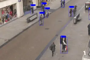
We had trained a lightweight SSD-MobileNet model using supervised learning on the Oxford Town Centre dataset, a dataset of videos from a public surveillance camera installed at the corner of Cornmarket and Market St. in Oxford, England. The model was light, fast, and worked well on all edge devices in real-time. However, when we used this model for inference in other environments, such as an office, a hospital, or even a street with a CCTV camera installed in a location and angle different from the training data, it performed poorly.

The reason was simple: the model was trained on the Oxford Town Centre dataset, with its specific characteristics. Since the data was specific to that environment, the model failed to generalize well to other unseen environments. We had two options here to tackle this problem:

1- Use several already labeled datasets to train a complex model, such as IterDet, that performs well in unseen environments. Then, apply that model to every new environment and (hopefully) get acceptable predictions.

2- For each new environment, gather and annotate data from scratch and use this dataset to train a lightweight model specific to that environment. We could also use a central server to reduce the training costs, i.e., for each new environment, send the data over the network to the server, annotate the data, train a new model using our fast server, and send the trained model back to the user.

However, none of these solutions were practical.

To work around the first solution, we needed to train a model that generalizes well to every unseen environment. However, reaching this goal was only possible through increasing the model complexity. Consequently, our application would need high-computational resources, and we could no longer process the (sensitive, private) data using the edge devices. Therefore, the application could not run in real-time, was expensive to use, and was not easily accessible everywhere. So, we decided to move to the next approach.

The critical issue with the second solution was privacy. If we wanted to have a central dataset where all the training happens, we needed to transfer huge amounts of sensitive data over the internet to our server, which is not safe, privacy-wise. What’s more, we didn’t have labeled data to train the model for each new environment, making this solution even harder to employ.

3. The Solution

Since we cannot train or run complex models on edge devices or moderate desktop computers, we need to move to the second solution, i.e., train a lightweight model for each new environment. But before doing this, we should resolve the issues with this solution that were related to user privacy and data annotation.

1- User Privacy: By applying some ideas in the training procedure (will be explained in detail), we can train the model locally and eliminate the need for a central server. We will also explain how we can train the model without storing any private data for long periods of time. Using these techniques, we no longer need to store or send private data over the internet, and user privacy will be preserved completely.

2- Data Annotation: For the sake of explanation, let us assume for now that we have a “magical annotation machine” that annotates data coming from every unseen environment, automatically. Isn’t the data annotation problem solved already? If we had such a machine, we would just need to train our lightweight model on our edge device using the pair of images and labels from each frame in the video. Fortunately, we already have the “magical annotation machine”.

In the next section, we will explain these ideas in more detail.

4- Adaptive Learning

The solution consists of two phases and works as follows:

4.1. Phase One: Training

In this phase, we go through these three steps:

STEP 1: We train a heavy, complex model to do the detection task. We call this model the Teacher Model (the reason behind this naming will be clear shortly). To train the teacher model, we need to have a rich, diverse dataset and design the model complex enough to perform well on data gathered from unseen environments. This step may take some time, but it only needs to be done once. For our pedestrian detection task, we used the IterDet model pre-trained on the Crowd Human dataset. This network acts as a teacher model for new environments.

STEP 2: We feed the new environment’s data to the teacher model to get the corresponding predictions. Here, we assume that the predictions are accurate enough to be used as ground truth labels for our images. Now, we have pairs of images and labels for each frame in our input video.

STEP 3: Using the pair of images and labels from STEP 2, we train a small, lightweight model on our edge device. We refer to this model as the Student Model.

4.2. Phase Two: Inference

We can now use the student model to run the application on our edge device with high accuracy. The teacher model can now be removed from the user’s computer to free up the disk storage.

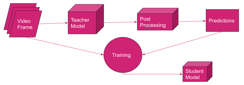
The whole adaptive learning process is illustrated in Figure 1. The training phase includes several rounds. For each round, we store a constant amount of data, say C frames, on the hard disk of the user’s computer. Then, we feed these C frames to the teacher model and obtain the corresponding labels to form C pairs of video frames and their labels. We will then use these C pairs of labeled data to train the student model. We remove these C pairs of data from the storage after they are loaded in the training pipeline and proceed to the next batch of frames, continuing from the last training checkpoint in every round.

4.3. Why Adaptive Learning?

There are several reasons why adaptive learning is a desirable solution to this problem. Here we mention some of the most important arguments:

1- Privacy: This is the first and most important reason. With adaptive learning, the teacher model runs on the user’s computer, and the student model runs on the edge device. So, everything is being processed locally, and no data needs to be stored permanently anywhere or transferred over the internet. Therefore, this approach preserves the user’s privacy and is completely safe.

2- No data annotation: By implementing this solution, you do not need to spend money and time on data annotation because the teacher model generates the labels automatically.

3- Speed: The lightweight student model is deployable on edge devices and runs in real-time, latency-free.

4- Accessibility: The most time-consuming part of adaptive learning is the training phase. However, the training phase only needs to be done once, and it takes a couple of days (at most) to finish. Afterward, we will have a lightweight model that runs on edge devices and is accessible everywhere.

To conclude, if the teacher model performs well, there is no bias in model predictions, and the student model trains well on data, adaptive learning works great.

You can find some benchmarks in Table 2 that measure mAP before and after applying adaptive learning to our pedestrian detection problem. For this example, we used the first 4500 frames of the video from the Oxford Town Centre dataset. We split these 4500 frames into training and validation sets with 3500 and 1000 frames in each set, respectively. The student model is trained on the first 3500 frames. Both baseline and adaptive learning student models are tested on the validation set with 1000 frames (from #3500 to #4500). Note that the student model is trained using the labels generated by the teacher model.

Method	mAP	Model
Baseline	25.02	SSD-MobileNet-V2 (trained on COCO)
Adaptive Learning	65.26	Teacher: IterDet (trained on Crowd Human), Student: SSD-MobileNet-V2

5. Challenges

We faced several challenges when we were trying to implement adaptive learning for our application. In this section, we mention some of these challenges and share the solutions we found.

5.1. Privacy Issues Related to Storing User Data

As we mentioned earlier, for each round, we feed C images (frames) to the teacher model to get the labels for each image. Since we want to use these C pairs of images and labels in the next step to train the student model, we should temporarily store these C pairs of labeled data on the user’s computer. Choosing a large value for C results in storing a large set of user’s data on storage for each round, consuming limited resources on edge and increasing privacy risks; on the other hand, assigning a small value to C leads to catastrophic forgetting, which brings us to the next challenge.

Through trial and error, we set C to an optimal value that prevents catastrophic forgetting while keeping the number of temporarily stored images low. Note that C is the number of frames that we are storing in each round, and these frames will be deleted from the user’s computer when loaded in the training pipeline.

We also applied some tricks to the code to get the most training out of the C selected frames. For example, we only keep those frames with a number of detected objects higher than a fixed threshold to end up with a rich set of training data while avoiding storing useless data. By applying all these techniques, we could build a minimal training set that is temporarily stored on the edge device, which minimizes privacy risks and concerns.

5.2. Catastrophic Forgetting

From Wikipedia,
Catastrophic interference, also known as catastrophic forgetting, is the tendency of an artificial neural network to completely and abruptly forget previously learned information upon learning new information.

Since we are training the student model in an online and incremental manner, the network is prone to catastrophic forgetting. To put it in simple terms, we are training the model in several rounds, and in each round, the model may forget what it has learned in the earlier rounds.

In an extreme case, suppose that we are training the model on data gathered from different hours of the day, and we are feeding the data to the model in chronological order. The network may simply forget the features it has learned from images taken in daylight when it reaches the night-time images.

We should especially be aware of catastrophic forgetting when applying online learning methods to a problem. According to the last section, the value that we choose for C can give rise to or avoid catastrophic forgetting. To further mitigate this issue, we can use an adaptive learning rate and reduce the learning rate in each round as the training progresses.

5.3. Network Instabilities

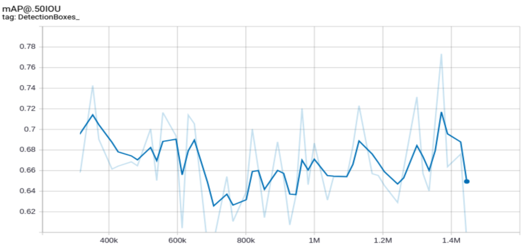
The model should train even on an ordinary computer with no GPU and no big RAM as an accessible solution. Thus, we need to apply several tricks to limit the training costs. For example, we should avoid using a large batch size because larger batch sizes require more memory. However, a small batch size creates network instabilities and causes some fluctuations in the training loss and training accuracy curves.
You can reduce the learning rate to keep the batch size small while avoiding fluctuations. In our case, when we trained the network with a batch size equal to one, we got the following mAP curve:

But after decreasing the learning rate, the curve was smoothed, as we see in the following figure:

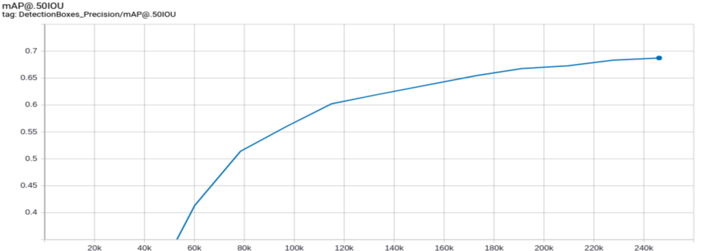
Although this approach works, it requires more time to converge. We suggest using gradient accumulation for faster convergence.

6. Improve the Accuracy Even More

So far, we have treated each frame as a separate image and processed the images independently rather than considering the temporal relation between the video frames. However, since the ultimate goal of this work is to process video feeds, taking the temporal dependencies into account during the training phase can increase accuracy. 

We conducted three different experiments to enter the temporal relation between video frames into the training process by manipulating the input image’s RGB channels. 

Note that there are lots of methods and model architectures in the literature that can capture temporal dependencies in video feeds in a sophisticated way. However, due to the model architecture limitations on edge (lightweight and easy to deploy on various edge devices), we could not use these methods and needed to apply other techniques to meet these limitations.

6.1. Background Subtraction:

In object detection applications where the objects of interest are moving, such as the Smart Social Distancing case, we can create a higher-level abstraction to detect the moving objects more efficiently using background subtraction. This pre-processing technique eliminates the estimated background from each frame to extract the moving objects (see Figure 4).

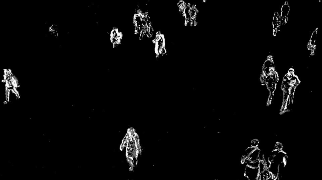
As you can see in the image above, by applying this algorithm, a mask is obtained that is active in pixels where the objects of interest (pedestrians) are present and inactive in other pixels.

To add this mask to the learning process, we replaced one of the RGB channels of the model’s input with this foreground mask.

6.2. Optical Flow

One of the most popular approaches to motion modeling in video feeds is the optical flow method.

We applied a dense optical flow algorithm to each video frame that returns the angle and magnitude of the flow vectors for each frame.

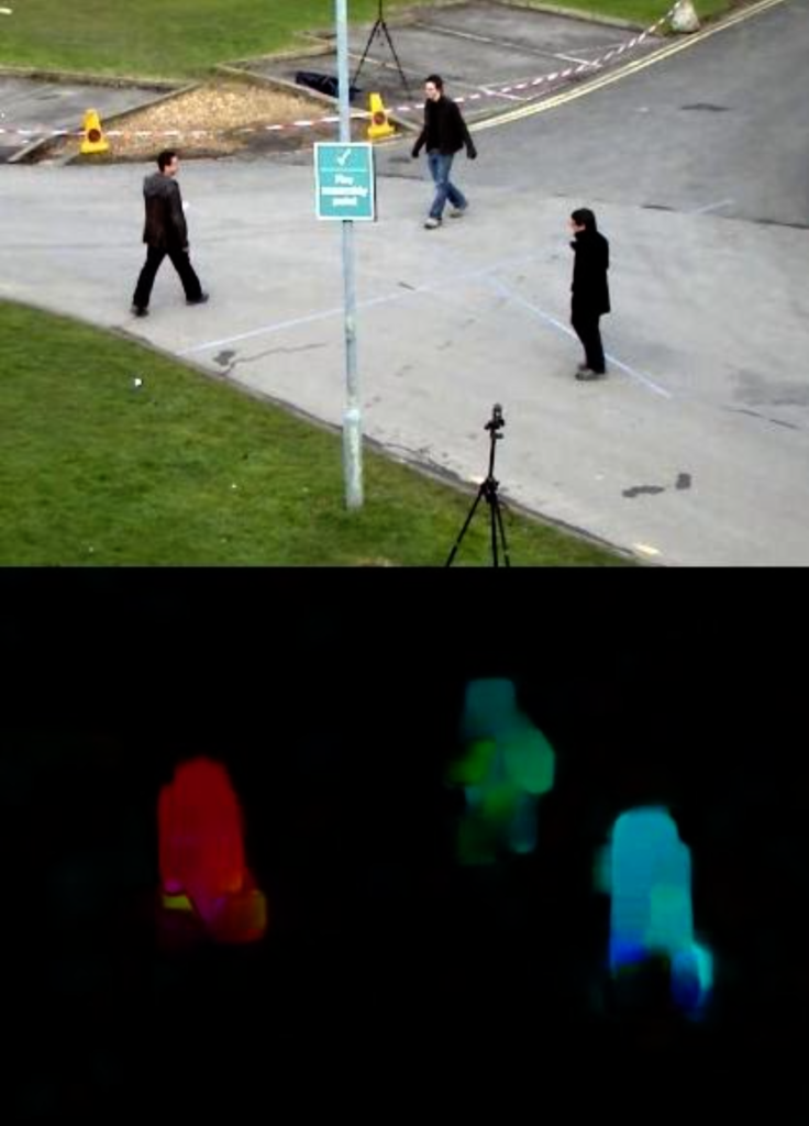
Since the angle of motion is not important in the object detection task, we discard this information and only keep the magnitude of the motion vector of each pixel in the form of a matrix. We embed the matrix of magnitudes into one of the RGB channels of the model’s input and train the student model with this supplementary information.

6.3. Combination of Background Subtraction and Optical Flow

In our last experiment, we combined the two previous techniques so that we embedded the foreground mask to one RGB channel of the model input and set the optical flow magnitude to another. For the remaining channel, we used the grayscale image of each frame to discard some color biases.

As you can see in Table 3, applying adaptive learning with background subtraction and optical flow can improve the mAP score by up to 72.2%, compared to the 25% mAP score at the baseline.

Model	mAP Score (%)
Adaptive learning with background subtraction	71.98
Adaptive learning with optical flow	70.56
Adaptive learning with gray scale image, background subtraction, and optical flow	72.20

7. Conclusion

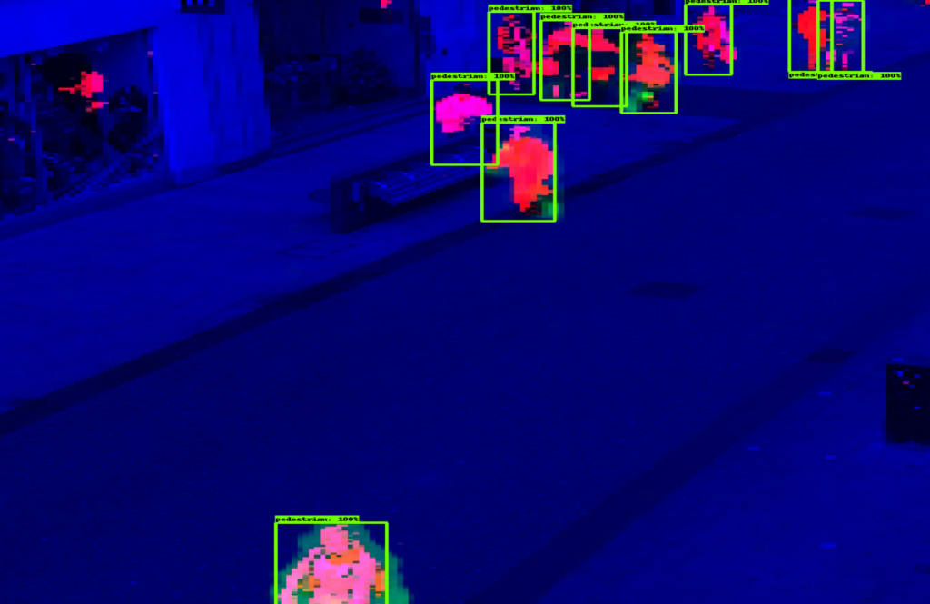
When designing the Smart Social Distancing application at Galliot, we applied Adaptive Learning to run the pedestrian detector in new environments. The results were impressive. You can compare the videos below to see the improvements (comparing the baseline on the left with adaptive learning on the right).

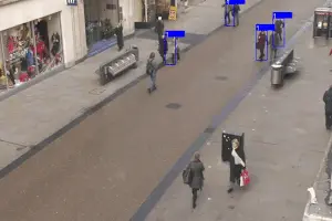
Suppose you need to do object detection in different environments. In that case, you can implement an adaptive learning method with a teacher-student configuration and train the student model for each environment separately. The student model will learn from the labels generated by the teacher model, so it relies on how accurately the teacher model labels the data. Aside from making sure that the teacher model labels the data with high accuracy, you need to solve several other challenges along the way, such as privacy issues related to storing user data, catastrophic forgetting, and network instabilities. Applying background subtraction and optical flow can further improve accuracy by ~7%.

You can get in touch with us for the Adaptive Learning API service and build your specialized object detection models easily. Feel free to contact us through the section provided below or via hello@galliot.us to ask for the service and further questions.