Month: September 2020
Smart Social Distancing: New Codebase Architecture
This tutorial provides a technical overview of the latest codebase architecture of the Galliot’s Smart Social Distancing application powered by AI on Edge.
This is Galliot’s solution for Detecting Social Distancing violations.
Visit our GitHub repository to read the application setup guide.
Read about the Data Labeling Methodologies and Solutions to learn how you can address your data requirements.
As a response to the coronavirus (COVID-19) pandemic, Galliot has released an open-source application that helps people practice physical distancing rules in different places such as retail spaces, construction sites, factories, healthcare facilities, etc. This open-source solution is now available as part of a standalone product at Lanthorn.ai.
This tutorial provides a technical overview of the approach to Smart Social Distancing. If you want to skip the implementation details, head to our GitHub repository to read the Smart Social Distancing application setup guide. You can read about our previous application architecture (outdated) in this article.
Note: Familiarity with deep learning computer vision methods, Docker, and edge deep learning devices, such as Jetson Nano or Edge TPU, is recommended to follow this tutorial.
1. Problem Description
Social distancing (also physical distancing) is one approach to control and prevent the infection rate of different contagious diseases, e.g., coronavirus and COVID-19, which is currently causing one of the largest pandemics in human history.
Wearing facemasks and maintaining social distancing are the most effective solutions to contain the spread of COVID-19. However, enforcing these policies poses a significant challenge to policymakers.
Please visit this blog post to read more about why current approaches fail and why we need a more robust approach.
2. Smart Social Distancing Application
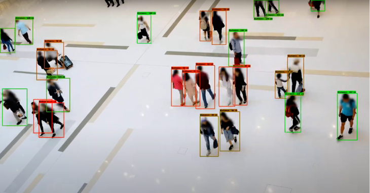
Our approach uses artificial intelligence and computing devices from personal computers to AI accelerators such as NVIDIA Jetson or Coral Edge TPU to detect people in different environments and measure adherence to social distancing guidelines. The Smart Social Distancing application provides statistics to help users identify crowded hotspots and can give proper notifications every time social distancing rules are violated.
2.1. A High-Level Perspective
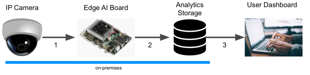
Smart Social Distancing application uses existing cameras to analyze physical distancing measures. The video will be streamed from a video feed to the main device, such as an Edge AI board or a personal computer. The main device processes the video and writes the analytical data on external storage. Analytical data only include statistical data, and no video or identifiable information is stored. Different graphs and charts visualize these statistics in the Dashboard. The user can connect to the Dashboard and view the analytical data, export it, and make decisions.
The user can access the Dashboard from a web browser. To ensure security and ease of development, requests to read the analytical data are sent directly to the main device by the web browser. As long as these requests and responses are encrypted, the Dashboard server cannot access the board’s stream and the analytical data. Since no data needs to be stored on the cloud, and no video file is stored on the analytics storage, the Smart Social Distancing application completely preserves the users’ privacy.
3. Codebase Architecture
We have achieved shippability and accessibility by “Dockerizing” the Smart Social Distancing application. The application architecture consists of two main parts that should be run separately; the Dashboard and the Processor.
The Dashboard consists of a React application served by a FastAPI backend, which provides the user with the necessary tools to communicate with the board and visualize the analytical data.
The Processor consists of an API and a Core; the Core is where the AI engine and the application logic are implemented. The API receives external commands from the user and communicates with the Core.
We will explain each component in more detail in the following sections.
3.1. Dashboard: an Overview
The Dashboard is where the visualizations happen; the user can find various charts and diagrams to better understand the measured statistics. The Dashboard interface is a React app served by a FastAPI backend.
The Dashboard consists of two Dockerfiles:
-
frontend.Dockerfile web-gui.Dockerfile
To run the Dashboard, you should build the frontend before building the web-GUI Dockerfile. Building the Dashboard is resource-intensive, and It is troublesome to build the Dashboard on devices with limited memory, such as Coral Edge TPU. Therefore, we have separated the Dashboard from the Processor to enable users to skip building the Dashboard if they wish to. However, the users would not encounter any problem building the Dashboard on other supported devices with higher capacities, such as X86 and most Jetson platforms.
Since the Dashboard is separated from the Processor, even if the Processor is not running, the user can still read the old statistics from the analytics server (of course, if the analytics server is accessible). However, any request to the Processor’s API will be failed, indicating that the Processor is not accessible at the time. On the other hand, regardless of whether the Dashboard is running or not, the Processor can run independently on the main device and store the statistics on the analytics storage. Users can access these statistics through the Dashboard at any time.
3.2. Technical Notes
If you plan to make changes to the web-GUI Dockerfile, you need to ensure that you are using the latest version of the frontend Docker image. Otherwise, some inconsistencies may occur.
3.3. Processor: an Overview
The application API, the AI core, and all the mathematical calculations to measure social distancing have been implemented in the Processor.
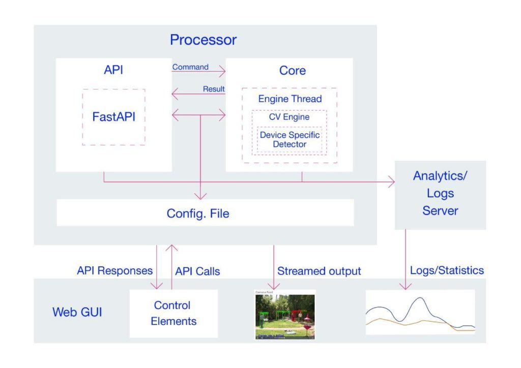
The Processor is made up of two main components; the Processor API and the Processor Core. The Processor API receives an API call from the outside world (the user) and sends a command to the Processor Core. The Core communicates with the API and sends the response according to the received command (if approved). Two queues, shared between the Core and the API, store the API commands and responses and enable the Core and the API to communicate.
Figure 2 illustrates the different components of the Processor. The arrows indicate the relations between these components. In the following sections, each component will be explained in more detail.
Processor Core
The Processor Core is where the AI engine and the application logic is implemented. The Core itself has several components and listens to the Processor’s API on a queue called the cmd_queuecmd_queue
Deep learning algorithms are implemented in a component named CvEngine (which is an alias for the Distancingcomponent in our implementation). CvEngine is responsible for processing the video and extracting statistical information. Note that some of the implemented algorithms, such as pedestrian detection, are device-specific, whereas other parts, extracting social distancing violations, for instance, are common between all the supported devices.
The Core keeps track of the tasks at hand and acts according to the received command. When the Core receives a command, it puts the proper response on a queue called the result_queueresult_queue for the response. Note that the Processor Core creates these queues, and the API registers them. If the Core component is not ready yet, the API will wait until the Core is up and ready and the queues are accessible. We will explain these commands and their responses in more detail in the following sections.
Processor API
The Processor API is where the external requests (by the user) are received. By these requests, we mean the supported API endpoints. Here is a list of supported commands with a description of what they do:
| API Endpoint | Description |
|---|---|
| PROCESSOR_IP:PROCESSOR_PORT/process-video-cfg | Sends command PROCESS_VIDEO_CFG to the Core and returns the response. It starts to process the video addressed in the configuration file. A true response means that the Core will try to process the video (with no guarantee), and a false response indicates that the process cannot start now. For example, it returns false when another process is already requested and running. |
| PROCESSOR_IP:PROCESSOR_PORT/stop-process-video | Sends command STOP_PROCESS_VIDEO to the Core and returns the response. It stops processing the video at hand and returns a true or false response depending on whether the request is valid or not. For example, it returns false when no video is already being processed to be stopped. |
| PROCESSOR_IP:PROCESSOR_PORT/get-config | Returns the config used by both the Processor’s API and Core. Note that the config is shared between the API and Core. This command returns a single configuration set in the JSON format according to the config-*.ini file. |
| PROCESSOR_IP:PROCESSOR_PORT/set-config | Sets the given set of JSON configurations as the config for API and Core and reloads the configurations. Note that the config is shared between the API and the Core. When setting the config, the Core’s engine restarts so that all the methods and members (especially those initiated with the old config) can use the updated config. This attempt will stop processing the video – if any. |
Some requests are directly related to the Core, such as process-video-cfgset-configCvEngine
3.4. Technical Notes
The start_services.bashrun_processor_core.pyrun_processor_api.py
To start processing the video by default when everything is ready, the sample_startup.bashprocess-video-cfg
3.5. Configurations
The Smart Social Distancing application uses two config files; config-frontend.iniconfig-*.ini
config-*.iniConfigEngineconfig-*.iniConfigEngine constructor. Therefore, they use the same configurations until a request is made by the user to set the config file.
When the set-configstop-process-videoprocess-video-cfgprocess-video-cfg
A key point about the config files is how to set the host and port. In config-frontend.iniProcessorApp section in this config file specifies the host and port on which the Dashboard is accessible. In config-*.iniconfig-frontend.ini
For example, let us say we want to run the Processor on port 2023, and for some customization reasons, we have changed the Processor’s Dockerfile so that the Processor API should use port 8040 inside the Docker (the default is on 8000). We should apply the following changes before running the application:
- Change the API port in
config-*.ini - Change the Processor port in
config-frontend.ini - Forward port 8040 of the Processor’s Docker to the
HOST_PORT
docker run -it --runtime nvidia --privileged -p 2023:8040 -v "$PWD/data":/repo/data -v "$PWD/config-jetson.ini":/repo/config-jetson.ini neuralet/smart-social-distancing:latest-jetson-nano
There are some other parameters that you can change in the config-*.ini[Detector]MinScoreDistThresholdconfig-*.ini
The config files are copied to the Docker images when they are built. Be aware that if you change the config files, you need to rebuild the Docker images to make sure the application is using the latest versions of the config files. The build time will be much less than the first time you build the Docker images because the copying will take place in the last layers of the Docker files. Therefore, the Docker images use the previously built Docker layers and only copy the necessary files into the new image.
4. The Application Logic
Most of the Smart Social Distancing application’s mathematical calculations are implemented in the Distancinglibs/distancing.pyDistancingcalculate_box_distances
We will now explain the building blocks of the Distancing
4.1. Image Pre-Processing and Inference
The __processDetector
By default, Smart Social Distancing uses SSD-MobileNet-V2 trained on the SAIVT-SoftBio dataset by Galliot for inference. Other possible models for your device are written as comments in the config file that matches your device name. In this file, you can change the Name parameter under the [Detector]
At Galliot, we have trained the Pedestrian-SSD-MobileNet-V2 and Pedestrian-SSDLite-MobileNet-V2 models on the Oxford Town Centre dataset to perform pedestrian detection using the Tensorflow Object Detection API. We experimented with different models on both Jetson Nano and Coral Dev Board devices. See Table 2 for more details.
| Device Name | Model | Dataset | Average Inference Time (ms) | Frame Rate (FPS) |
|---|---|---|---|---|
| Jetson Nano | SSD-MobileNet-V2 | COCO | 44 | 22 |
| Coral Dev Board | SSD-MobileNet-V2 | Oxford Town Centre | 5.7 | 175 |
| Coral Dev Board | SSD-MobileNet-V2-Lite | Oxford Town Centre | 6.1 | 164 |
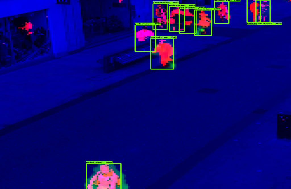
4.2. Bounding Box Post-Processing
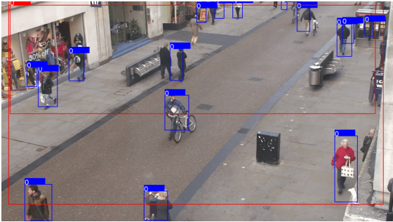
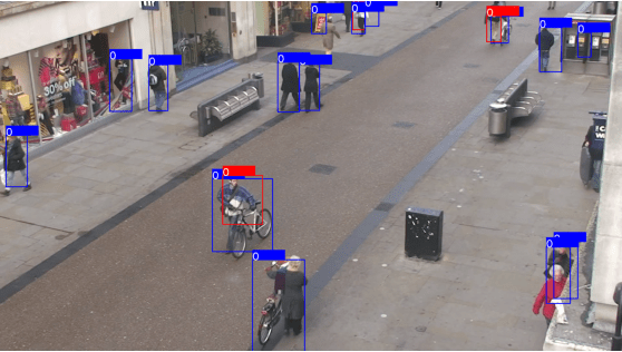
Some post-processing techniques are applied to the detected bounding boxes before calculating distances to minimize errors. There are some reasons to apply post-processing techniques. First, since we are using a general-purpose object detection model trained on COCO with 80 different classes, including pedestrians, there are some false positive outputs for the pedestrian detection task. These false positives are often seen in the form of extra-large boxes (Figure 3) or duplicate boxes specifying a single object (Figure 4). In the following lines of code, we address these two problems by filtering large and duplicate boxes:
new_objects_list = self.ignore_large_boxes(objects_list)
new_objects_list = self.non_max_suppression_fast(new_objects_list,
float(self.config.get_section_dict("PostProcessor")["NMSThreshold"]))
The second reason to apply post-processing is to track objects smoothly. In the absence of post-processing, the object detection model may lose track of the detected pedestrians from one frame to the other. This issue can be solved by designing a tracker system that follows the detected pedestrians in different frames.
tracked_boxes = self.tracker.update(new_objects_list)
4.3. Calculating Distances
The __processcalculate_distancing
There are a few methods to calculate the distance between two rectangles; however, choosing the right approach to measure this distance depends on different specifications, such as the data characteristics and the camera angle. Since some measures, such as the distance between the camera to the center of the bounding boxes or the depth data, are not available in most cases, we implemented a calibration-less method as well as a calibrated one. The calibrated method is more accurate than the calibration-less method. However, the latter is easier to implement. Let us explain more about each method.
Calibration-less Method
In this approach, we map the distances in the image (in pixels) to physical distance measures (in meters), by assuming that each person is H = 170 cmLL1L2L3L4
1- Assume that L = L1 = L2 = L3 = L4
2- Assume that L = min (L1, L2, L3, L4)
Following the first assumption makes the approach easier to understand with fewer amount of calculations needed. However, the second method produces more accurate results.
We explain how to calculate L1 in this section. If you want to use the first method, put L = L1L by setting it equal to the minimum value of L1L4. It is trivial that you can calculate L2L3L4
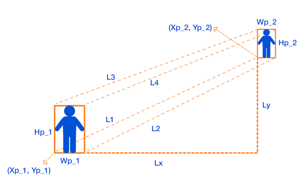
To measure L1DXDY
DX = Xp_1 - Xp_2
DY = Yp_1 - Yp_2
Then, by the H = 170 cm
Lx = DX * ((1 / H1 + 1 / H2) / 2) * H
Ly = DY * ((1 / H1 + 1 / H2) / 2) * H
Finally, we apply the Pythagorean formula to get L1:
L1 = sqrt(Lx + Ly)
We can now calculate L
In your device config file,
– You can set the DistMethodPostProcessorCenterPointsDistanceFourCornerPointsDistanceLL = min (L1, L2, L3, L4)
– The minimum physical distancing threshold is set to 150 centimeters by default. You can set a different threshold for physical distancing by changing the value of DistThreshold
Calibrated Method
The calibrated method takes in a homography matrix and calculates the real-world distances by transforming the 2D coordinates of the image to the real-world 3D coordinates. We will explain how this method works in a separate post.
4.4. Data Visualizations
Some data visualizations are provided to give the user better insights into how well physical distancing measures are being practiced. The data analytics and visualizations can help decision-makers identify the peak hours and detect the high-risk areas to take effective actions accordingly.
The visualizations include a camera feed, a birds-eye view, the pedestrian plot, and the environment score plot.
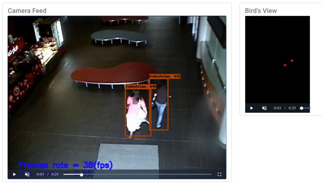
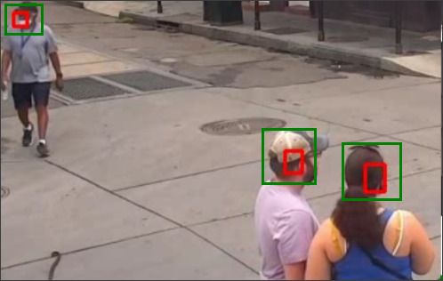
Camera Feed
The camera feed shows a live view of the video being processed (see Figure 6). Colored bounding boxes represent detected pedestrians. You can see the frame rate and environment score (explained below) at the bottom of the video screen.
Birds-eye View
This video shows the birds-eye view of the detected pedestrians (see Figure 6). The red color indicates a social distancing violation, while the green color represents a safe distance between the detected pedestrians in each frame.
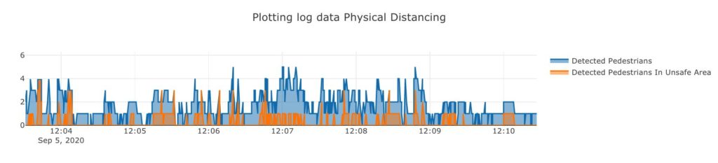
Pedestrian Plot
The pedestrian plot (Figure 7) shows the total number of detected pedestrians (the blue graph) and the number of detected pedestrians who are violating the physical distancing threshold (the orange graph) over time.
Environment Score Plot
This plot (Figure 8) shows the “environment score” over time. The environment score is an index defined to evaluate how well social distancing measures are being practiced in an environment. Two different formulas are implemented to measure the environment score in tools/environment_score.py
1- The mx_environment_scoring
env_score = 1 - np.minimum((violating_pedestrians / MAX_ACCEPTABLE_CAPACITY), 1)
Note that MAX_ACCEPTABLE_CAPACITYDistThresholdMAX_ACCEPTABLE_CAPACITY
2- The mx_environment_scoring_consider_crowd
env_score = 1 - np.minimum(((violating_pedestrians + detected_pedestrians) / (MAX_CAPACITY + MAX_ACCEPTABLE_CAPACITY)), 1)
In this formula, the MAX_CAPACITY
Note that in both formulas, the environment score takes a value between 0 to 1, and the more violating cases appear in a frame, the less the environment score of that frame becomes.
4.5. Data Logging System
We have implemented a logging system for the Smart Social Distancing application that can be very useful for data analytics. By storing statistical data, such as the overall safety score, the number of people in the space over the past day, and total risky behaviors, users can gain insights into different social distancing measures. Let us explore how the logging system works.
There are three files under the libs/loggerscsv_processed_logger.pycsv_logger.pyloggers.py
The first two scripts implement their update method that is called from the loggers.pyupdate
NameTimeIntervalLogDirectory
The update method in the csv_processed_logger.py
The csv_logger.py
- The object log keeps track of the information about all the detected objects in each time interval. Frame number, person id, and bounding box coordinates are stored in this log file.
- The distance log stores the details of physical distancing violation incidents, such as the time in which physical distancing rules are violated, the id of the persons crossing the distance threshold, and the distance they are standing from each other.
Please reach out to hello@galliot.us if you have any questions. Check out our GitHub page for other models and applications by Galliot.
Real-world Face Mask Detection Part1; Problem Statement

image source freepik.com
In this article, we cover the mask detection problem, details about our synthetic ddataset, and classifier that can identify if people are wearing a face mask or not in real-world scenarios.
This is the first part of a two-part series on real-world face mask detection by Galliot.
Skip to the second part to see how we built a Face Detector working on real-world data.
Visit our Solutions Page to see other solutions by Galliot.
Read our Guide to Data Labeling article to learn about different approaches for handling labeling needs.
Wearing a mask in public settings is an effective way to keep the communities safe. As a response to the COVID-19 pandemic, we open-sourced a face mask detection application created by Galliot that uses AI to detect if people are wearing masks or not. We focused on making our face mask detector ready for real-world applications, such as CCTV cameras, where faces are small, blurry, and far from the camera.
This series has two parts; In this post, we present a series of experiments we conducted and discuss the challenges we faced along the way. We also cover the details about our mask/no-mask classifier. In part 2, we will go over building a face detector that can also detect small faces in real-world data. We will also deploy our face mask detector on edge and explain some code base configurations.
We have published our dataset (click to download) and our trained face mask detector model to share the results with the community.
1. Mask Detection Problem statement
Before getting started, let us understand the problem better. We want to build a system that can detect faces in real-world videos and identify if the detected faces are wearing masks or not. So, what do we mean by real-world videos?
If you look at the people in videos captured by CCTV cameras, you can see that the faces are small, blurry, and low resolution. People are not looking straight at the camera, and the face angles vary from time to time. These real-world videos are entirely different from the videos captured by webcams or selfie cameras, making the face mask detection problem much more difficult in practice.
In this blog post, we will first explore mask/ no mask classification in webcam videos and next, shift to the mask/ no mask classification problem in real-world videos as our final goal. Our reported model can detect faces and classify masked faces from unmasked ones in webcam videos as well as real-world videos where the faces are small and blurry and people are wearing masks in different shapes and colors. We will explain more details about the face detector in the next part.
2. The inspiration
Several online sources for face mask detection are currently available on the internet, such as this post by Adrian Rosebrock from PyImageSearch. These systems can detect face masks in videos where people are placed in front of the camera. Here is a demo video by PyImageSearch that shows how this system works in practice:
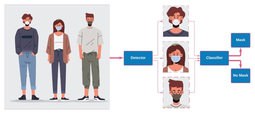
Since no dataset annotated for face mask detection is currently available, a model cannot be trained to detect faces and do a mask/ no mask classification simultaneously. Thus, most current solutions divide the face mask detection system into two sub-modules; 1- the face detector and 2- the mask / no-mask classifier. The detector detects faces in the video stream, regardless of wearing a mask or not, and then outputs bounding boxes that identify the faces’ coordinates. Next, the detected faces are cropped and passed to the classifier. Finally, the classifier decides if the cropped face is wearing a mask or not.
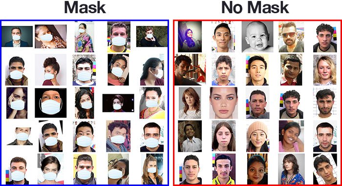
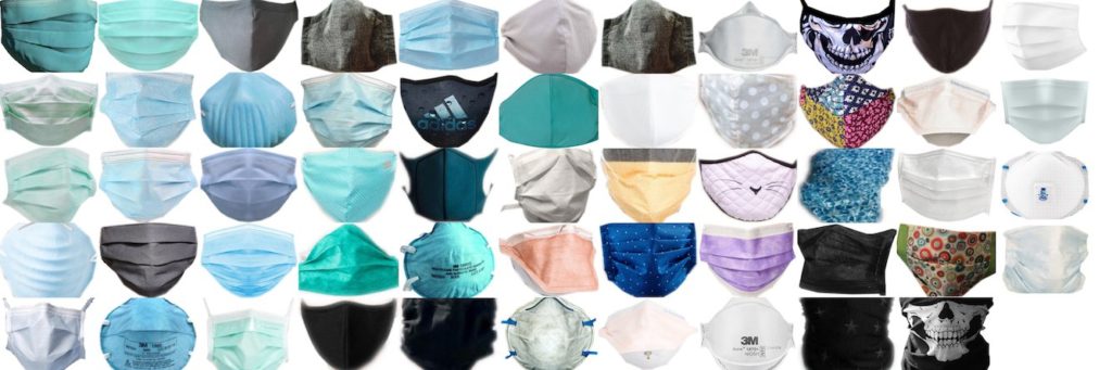
For example, in the mentioned post by PyImageSearch, a Single Shot MultiBox Detector (SSD) pre-trained on the WIDER FACE dataset is used for face detection. Also, to perform mask/ no mask classification, a synthetic dataset is used to train a MobileNet-V2 classifier. This dataset contains images from both mask and no mask classes with nearly 1400 images. The masked faces are synthesized by artificially adding surgical face masks to normal faces. We will refer to this dataset as “SM-Synthetic (SurgicalMask-Synthetic)” throughout the rest of this post. Here is an example of the images from SM-Synthetic:
In the example from PyImageSearch, the MobileNet-V2 classifier was trained on SM-Synthetic with 99% accuracy on the validation set. However, in most real-world applications, the faces are far from the camera, blurry, and low resolution. Unfortunately, this dataset cannot help us solve the problem in such cases.
Moreover, currently available datasets for face mask classification only include a few face mask types. For example, the only face mask used in the SM-Synthetic dataset is a plain, white surgical mask. In practice, however, people use different kinds of face masks in every color and various shapes. A face mask classifier trained on the SM-Synthetic dataset fails to generalize well to different face masks due to the lack of diversity. In the following video, you can observe that the model fails to classify unseen face masks correctly:
Compare this demo with our final classifier:
At Galliot, we were curious about building a face mask detector that can generalize well to real-world data. We tried different datasets with several detectors and classifiers to come up with the right solution. In the following series of experiments, we will walk you through the evolutionary path that we followed to construct a real-world mask/ no mask dataset and build a face mask classifier that can also work well on real-world data.
For convenience, the details about all datasets that we will refer to throughout this post are listed in Table 1.
| Dataset Name | Dataset Size | Training Set | Validation Set | Description |
|---|---|---|---|---|
| SM-Synthetic | 1457 | Mask: 658 No Mask: 657 | Mask: 71 No Mask: 71 | Link to the dataset A surgical mask is synthesized on faces. |
| BaselineVal | 2835 | – | Mask: 1422 No Mask: 1413 | Collected from CCTV video streams with blurry, low-resolution images. |
| Extended-Synthetic / Extended-Synthetic-Blurred | 23K | Mask: 9675 No Mask: 10353 | Mask: 1206 No Mask: 1207 | Link To the dataset. Collected from WIDER FACE, CelebA, and SM-Synthetic. Fifty-four distinct face masks are synthesized for normal faces. |
| FaceMask100K | 100K | Mask: 50604 No Mask: 49417 | Mask: 1422 No Mask: 1413 | Collected from CCTV video streams with blurry, low-resolution images. Manually labeled by Galliot. |
3. Experiment #1: The First Shot
For the first experiment, we trained an SSD-MobileNet-V1 model to reproduce the work by PyImageSearch. The face detector was trained on WIDER FACE, a face detection benchmark dataset, and achieved a 67.93% mAP score on the WIDER FACE validation set. We used the SM-Synthetic dataset to train a mask/not mask MobileNet-V1 classifier that achieved 99% accuracy on the SM-Synthetic validation set.
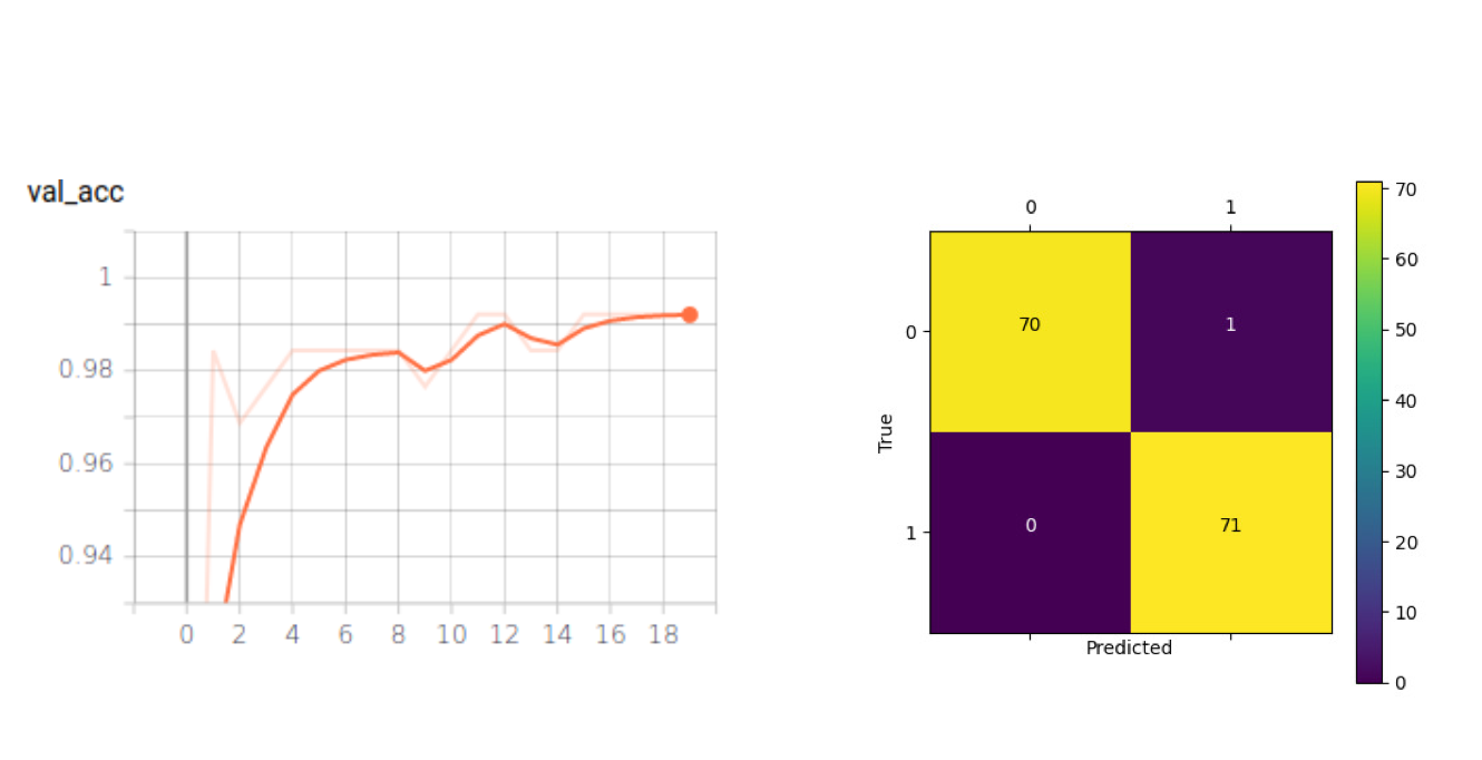
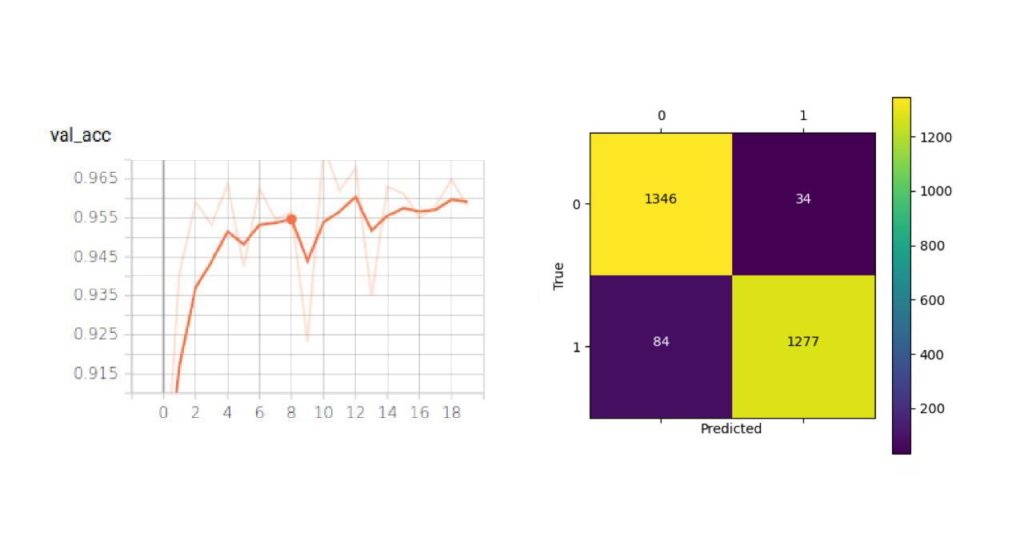
Then, to cut the number of parameters used by the MobileNet-V1 classifier model (~3.5 M parameters), we started thinking about whether we could build a custom CNN model that can do the same task as well as the previous model using much fewer parameters. After some experiments, we created the optimized CNN model, called OFMClassifier (Optimized Face Mask Classifier), with ~296K parameters – about 12x fewer than the number of parameters in the MobileNet-V1 model. This model achieved 99% accuracy on the resized version of the SM-Synthetic validation set (see Figure 3) 8x faster than the MobileNet-V1 model on GeForce RTX 2070 Super (see Table 2).
| Classifier | Inference time (ms) |
|---|---|
| MobileNet-V1 | 9.7 |
| OFM-Classifier | 1.2 |
Since the OFMClassifier worked as well as the MobileNet-V1 model using much fewer parameters, we decided to choose this network over the MobileNet-V1 model for this experiment.
We will train this model on different datasets throughout the rest of this post. The network architecture is explained in more detail in the following section.
3.1. Network Architecture Details and Hyperparameters (for Experts)
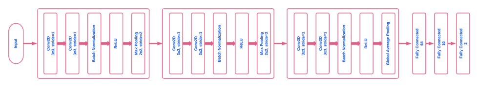
The network architecture is illustrated in Figure 4. The OFMClassifier model has three convolutional blocks. Each block has two consecutive convolutional layers followed by a “max pooling” and a “dropout” layer. In the convolutional layers, padding is added to input data to preserve image resolution and spatial size. Also, batch normalization is applied to ensure network stability. We applied max pooling to reduce image resolution, and in the last layers, we used global average pooling instead of using the flatten layer to perform down-sampling with fewer features (128 instead of 11*11*128). Finally, two fully connected layers are added to the network for the purpose of mask/ no mask classification (mask/ no mask).
For all the experiments, we applied the “Adam” optimizer with a learning rate of 0.0002, and the loss function was categorical cross-entropy. We used a batch size of 16 and trained our network for 20 epochs.
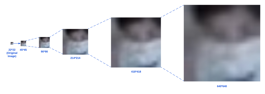
3.2. A Note On the Network Input Shape
Detected faces are cropped out of the original image before being passed to the classifier; therefore, they are already small. If we wanted to use large input shapes, we had to enlarge the detected faces, which would result in losing some useful information (see Figure 5). Also, we could minimize the computations and achieve faster inference by keeping the image size small. Thus, we changed the input shape to 45*45 pixels before passing the images to the network.
3.3. Experiment #1: the results
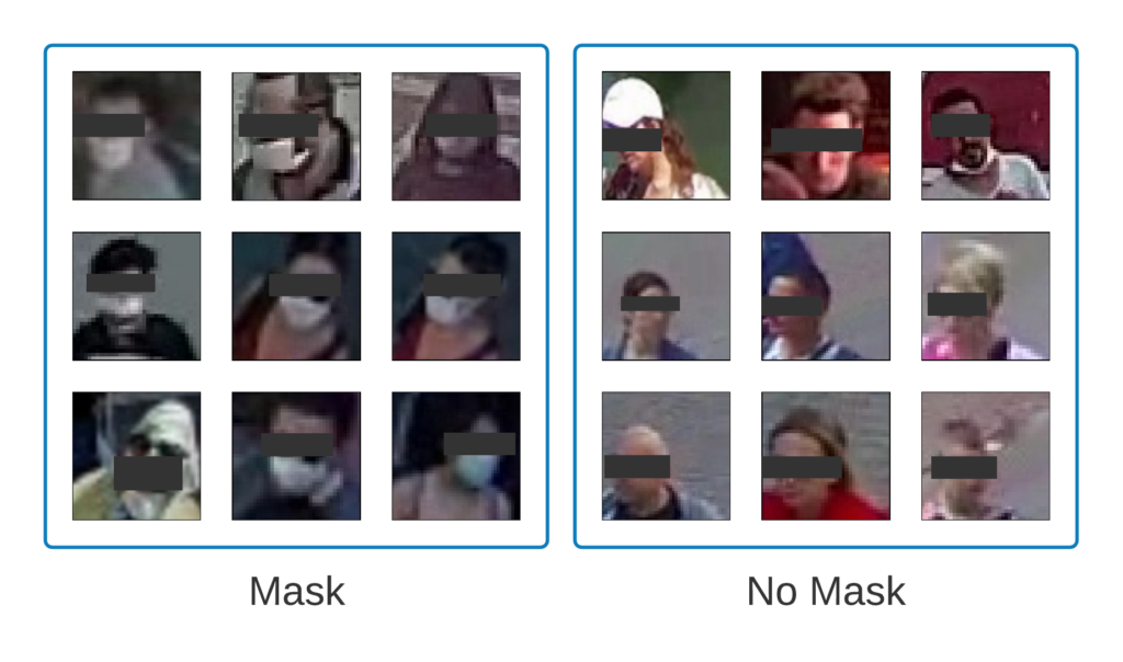
The model achieved 99% accuracy on the validation set, but don’t get too excited (yet)! To investigate if the OFMClassifier can generalize well to real-world data with blurry, low-resolution faces that are further from the camera, we constructed another validation set called BaselineVal. This dataset contains 2835 images belonging to two classes (mask/ no mask) collected from CCTV video streams. Figure 6 shows some examples from the BaselineVal dataset.
We tested the OFMClassifier on BaselineVal, and the model was degraded to an almost-random guesser with 62% accuracy. Figure 7 illustrates the new validation accuracy curve and the confusion matrix (compared with Figure 3).
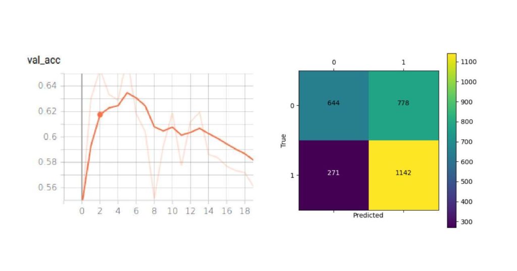
The OFMClassifier that worked well on the SM-Synthetic validation set failed to generalize to real-world data. We think that the main challenge is creating a more representative dataset with more diversity.
4. Experiment #2: The Extended-Synthetic Dataset
Following the previous experiment, we started synthesizing a new dataset from scratch, this time with more mask types in different colors and textures, to see if adding more diversity to face masks can improve model accuracy. We took normal face images from WIDER FACE, and CelebA artificially added face masks to these faces and added some images from the SM-Synthetic dataset to create the Extended-Synthetic dataset. The Extended Synthetic dataset is available for download here. Figure 8 illustrates the 54 different kinds of face masks that we used to build this dataset. A dataset of 54 different kinds of facemasks in .PNG format is available for download here. We also synthesized these face masks to 50K images from the CelebA dataset, which is available for download here.
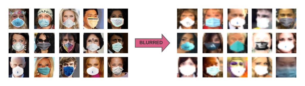
To make our dataset comparable to real-world scenarios, we blurred the faces from Extended-Synthetic to create a new dataset named Extended-Synthetic-Blurred with the same number of images in both training and validation sets. You can compare Extended-Synthetic-Blurred with Extended-Synthetic (not blurred) in Figure 9.
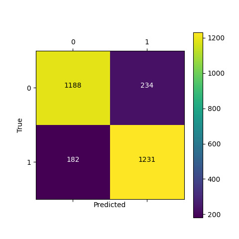
We used the SSD-MobileNet-V1 model from the previous experiment as the detector and trained an OFMClassifier on the Extended-Synthetic-Blurred dataset to classify the detected faces to mask/no mask classes. Figure 10 illustrates the validation accuracy curve and the confusion matrix for this experiment.
The model converged with 95% accuracy on the Extended-Synthetic-Blurred validation set.
To compare the classification accuracy between this model and the one from the first experiment, we also evaluated this model (trained on the Extended-Synthetic-Blurred dataset) on the BaselineVal dataset. The model outperformed the network trained on the SM-Synthetic dataset with 62% accuracy from experiment #1 (see Figure 7) and achieved 85% accuracy on the BaselineVal dataset.
We also tested this model on the demo video from experiment #1. You can see how adding images from several mask types to the training data can improve classification accuracy:
Furthermore, this model achieved a high accuracy of 96% when evaluated on the SM-Synthetic validation set. We can observe that this model outperforms the model from experiment #1 on BaselineVal while performing almost as accurately on the SM-Synthetic validation set.
Conclusion: Combining real-world data with blurred synthesized data that contains several mask types in different shapes, colors, and textures, increases model generalizability.
We trained a model on a synthetic dataset that achieved 95% accuracy on its validation set, which is pretty good. We also evaluated this model on the BaselineVal dataset –constituted of real-world data with no synthetic images– and the model obtained 85% accuracy. According to these results, we can conclude that the classification problem is more difficult with real-world data.
We examined the possible solutions to the mask/ no mask classification problem using synthetic datasets, but we were still looking for a production-level model trained on real-world data. Thus, we decided to manually annotate a dataset that represents real-world scenarios for mask/ no mask classification.
5. Experiment #3: FaceMask100K
We used several sources, such as videos from CCTV cameras, to construct a dataset with images representing real-world scenarios. The images were annotated with class names (mask/ no mask). The created dataset, called FaceMask100K, contains 98542 images in the training set and 2835 images in the validation set belonging to two classes (mask/ no mask).
Annotating this dataset required much effort. We collected videos from CCTV cameras captured in different places over several hours of the day and trimmed out those frames where a few people were passing by. Since the faces were too small in these videos, detecting faces was challenging, and common face detection approaches, such as training an SSD-MobileNet detector, did not work. Therefore, we used OpenPifPaf to detect faces and then extracted human heads (according to OpenPifPaf “Keypoints”) from these frames. Then, we manually annotated the detected faces to mask/ no mask classes. We will explain face detection challenges in CCTV video streams in more detail in part 2 of this series.
We trained a classifier on FaceMask100K that achieved 98% accuracy on the training set and 92% accuracy on the BaselineVal dataset, outperforming all the models from previous experiments. This model also achieved 97% accuracy on the SM-Synthetic validation set, 96% accuracy on the Extended-Synthetic validation set, and 95% accuracy on the Extended-Synthetic-Blurred validation set. Table 3 lists the datasets that we used to train the classifiers discussed in this post with their classification accuracy on the BaselineVal dataset.
| Training Dataset | Classification Accuracy on the BaselineVal Dataset |
|---|---|
| SM-Synthetic | 62% |
| Extended-Synthetic-Blurred | 85% |
| FaceMask100K | 92% |
6. Results
In the following table, you can see three face mask detectors by Galliot tested on different videos. The model trained on the Extended Synthetic dataset is the best when you want to detect face masks in videos with high quality, and the model trained on FaceMask100K is suitable for face mask detection on CCTV videos.
| Dataset Name | Demo Video #1 |
|---|---|
| Surgical Mask Synthetic | https://www.youtube.com/embed/a8C05FKbqQs |
| Extended Synthetic Blurred | https://www.youtube.com/embed/vRCeTMI4zeU |
| FaceMask100K | https://www.youtube.com/embed/pPEhfbskMTg |
| Dataset Name | Demo Video #2 |
|---|---|
| Surgical Mask Synthetic | https://www.youtube.com/embed/-lnacGf09WI |
| Extended Synthetic Blurred | https://www.youtube.com/embed/hvhc7dDpHMY |
| FaceMask100K | https://www.youtube.com/embed/M7wltRbEgIg |
| Dataset Name | Demo Video #3 |
|---|---|
| Surgical Mask Synthetic | https://www.youtube.com/embed/pWkexuP_IVs |
| Extended Synthetic Blurred | https://www.youtube.com/embed/Ti3Li4kvTmg |
| FaceMask100K | https://www.youtube.com/embed/n42lEDFkfbs |
7. Challenges
There are some cases in which our model has trouble classifying masked faces from unmasked ones correctly. For example:
– In some cases, the classifier changes its prediction for one detected face a few times. Adding a voting system or applying a tracker can improve the classification.
– We focused on creating a diverse training set. However, the training data does not have enough examples of some environmental conditions, such as lighting settings. For instance, there are not too many examples captured during the nighttime in the training set. Therefore, the model misclassifies some faces in videos captured at night. Adding more data to the dataset can improve classification accuracy in such cases.
– Our classifier struggles with classifying some face mask types. For example, red masks are often misclassified. Adding more face masks to the training data can fix this issue.
– The model cannot correctly classify masked faces from unmasked ones when the faces are too blurry, especially in cases where even a human cannot identify whether the person is wearing a mask or not.
– The model misses some faces and fails to classify face masks in videos that are captured from unseen angles. For example, the model cannot perform well in overhead angle views.
In future attempts, we will try to further improve our classifier and mitigate the mentioned challenges.
8. Conclusion
Because of data limitations, current approaches to building a face mask detector system are composed of two sections: the face detector and the mask/ no mask classifier. This post focused on training a mask/ no mask classifier that can work in real-world scenarios. In the next part, we will explain how to train a detector to detect small, blurry faces.
To train a mask/ no mask classifier, we started by training a model on an open-source synthetic dataset with much fewer parameters than a MobileNet model while preserving accuracy. Then, to add more diversity to the data, we created a new, larger dataset, called the Extended-Synthetic dataset, with 54 different mask types and blurred the faces to obtain Extended-Synthetic-Blurred. We trained a model on the blurred dataset, and the model outperformed the one from the previous experiment by a large margin. Then, to further improve our results and build a production-ready classifier, we built FaceMask100K, a large-scale dataset constituted of real-world mask / no mask images. We trained a CNN classifier on FaceMask100K that achieved 92% accuracy on the validation set and reported this model as our best face mask classifier. To the best of our knowledge, this model outperforms all the currently available face mask classifiers that can work on CCTV video streams. Our demo videos show that this model can work pretty well in real-world scenarios.
To facilitate continued work in this space, we have open-sourced the Extended Synthetic dataset. You can download the dataset by clicking on this link. Galliot’s face mask detection models are available for download on our GitHub repo. Select and download the model according to the platform you are using:
Refer to the second part of this article to learn more about the face detector we used in this application. Do not forget to check out our GitHub repo and other blog posts on our website to learn more.
License
This project is sponsored by Lanthorn. Visit Lanthorn.ai to learn more about our AI solutions.
All released datasets (Extended Synthetic dataset, Neuralet FaceMask50K dataset), released models, and Galliot’s GitHub source code are licensed under the Creative Commons Attribution-NonCommercial-ShareAlike 4.0 International License.

Please reach out to us via hello@galliot.us or the contact us form if you need to use the datasets, model, or code base for commercial purposes; we are happy to help you!
Introducing Lanthorn.ai
Lanthorn.ai
Lanthron.ai is a Video analytics decision support tool to control workplace risk and safety – The Future of Occupancy Analytics & Surveillance
Combat COVID-19 With AI-Enabled Video Analytics: Introducing Lanthorn.ai
Businesses, regardless of industry, are facing a mountainous task when it comes to the creation of a safe environment for their employees and customers. The current approach to mitigating the risk of COVID-19 is archaic and relies on solutions such as stickers on the ground and human supervision.
Lanthorn.ai is here to help businesses -from manufacturing and retail to sports and recreational venues- reduce their risk using the power of AI-enabled Video Analytics. By using Lanthorn.ai, you can predict and mitigate the risk of COVID-19 transmission.
Our unique algorithm is trained to detect:
- The number of people in a space to determine occupancy;
- The distance between people to uncover social distancing violations; and
- Mask usage to uncover unsafe practices.
The data gathered using our AI algorithm is displayed on Lanthorn.ai’s Dashboard, which gives you insights into:
High-Risk Hours – Lanthorn.ai can assess what hours a location has the most number of violations; so that your business can redistribute traffic and reduce the number of violations.
High-Risk Locations – Lanthorn.ai can identify the areas with the most number of social distancing and mask usage violations and thereby infer which teams need more training to follow COVID-19 protocols.
Comparative Data – By using Lanthorn.ai, you can see how many violations of COVID-19 protocols there are before and after safety training and precautions.
Our Dashboard can be customized to send you alerts using email, text, or other notification platforms. This means you do not have to monitor the Dashboard in order to know when and where you have hotspots.
Lanthorn.ai works by using your existing video feeds. It can process video feeds without ever sending your data outside of your network.
For more information, visit our website, www.lanthorn.ai, or contact us at hello@lanthorn.ai
Adaptive Learning Computer Vision
Image Source: https://imgur.com/rDTXu
Adaptive learning builds robust systems that adapt to novel data distributions without having to store or transfer data from edge devices to other systems.
Here is Galliot’s Adaptive Learning tutorial for building object detection models.
You can contact us for Edge Vision API service to try this solution and build your first specialized model.
Building robust computer vision models requires high-quality labeled data. Read more about how to handle your data labeling needs.
Adaptive Learning aims to build robust systems that can work efficiently and adapt to new environments (novel data distributions) without having to store or transfer data from edge devices to other systems. When applied, this will dramatically simplify machine learning systems’ architecture and lower their deployment and maintenance costs.
We present adaptive learning as a solution to train a lightweight pedestrian detection model that performs well on unseen data. We will explain the benefits of adaptive learning and discuss some challenges along the way. We will also review some optimizations to further improve model performance.
1. Overview
Let’s suppose you want to train an object detection model. Depending on your specific needs, you may decide to follow one of the following approaches:
1- Train a highly accurate and generalizable but computationally heavy model such as FasterRCNN
2- Train a lightweight but not a generalizable model like SSD-MobileNet
What is the trade-off here?
Go with the first approach and train a heavy network. You will have to sacrifice speed for accuracy, i.e., the model will provide strong generalization with relatively high accuracy at the cost of large memory and compute footprint. It will demand high-computational resources during both training and inference phases and cannot be deployed on edge devices that have limited memory and computational power.
What if we follow the other approach and train a lightweight model? As you have probably guessed the right answer, the predicted output will be less accurate and cannot generalize well on new, unseen data from other environments. That is because the lightweight model is using fewer parameters to do the computations, and the network architecture is also less complex. However, if you train a lightweight model on data gathered from one environment, the model will perform well on unseen data coming from the same environment. Furthermore, the model will run faster, will not impose high computational costs, and can be deployed on edge devices that run applications in real-time, minimizing latency.
| Heavy Models | Lightweight Models |
|---|---|
| Higher accuracy | Less (but still acceptable) accuracy |
| Generalize well on unseen environments | Fail to generalize well on unseen environments |
| non-real-time inference | Real-time inference |
| High computational costs | Minimum computational costs |
| Cannot be deployed on edge devices | Can be deployed on edge devices |
For those applications that are constrained by time and computing resources, we have no option but to use the second approach and train a lightweight model. Therefore, we should look for some techniques to adapt the lightweight model to different environments while improving model accuracy.
2. The Problem
We encountered a similar problem at Galliot when we were working on our open-source Smart Social Distancing application.
We had trained a lightweight SSD-MobileNet model using supervised learning on the Oxford Town Centre dataset, a dataset of videos from a public surveillance camera installed at the corner of Cornmarket and Market St. in Oxford, England. The model was light, fast, and worked well on all edge devices in real-time. However, when we used this model for inference in other environments, such as an office, a hospital, or even a street with a CCTV camera installed in a location and angle different from the training data, it performed poorly.
The reason was simple: the model was trained on the Oxford Town Centre dataset, with its specific characteristics. Since the data was specific to that environment, the model failed to generalize well to other unseen environments. We had two options here to tackle this problem:
1- Use several already labeled datasets to train a complex model, such as IterDet, that performs well in unseen environments. Then, apply that model to every new environment and (hopefully) get acceptable predictions.
2- For each new environment, gather and annotate data from scratch and use this dataset to train a lightweight model specific to that environment. We could also use a central server to reduce the training costs, i.e., for each new environment, send the data over the network to the server, annotate the data, train a new model using our fast server, and send the trained model back to the user.
However, none of these solutions were practical.
To work around the first solution, we needed to train a model that generalizes well to every unseen environment. However, reaching this goal was only possible through increasing the model complexity. Consequently, our application would need high-computational resources, and we could no longer process the (sensitive, private) data using the edge devices. Therefore, the application could not run in real-time, was expensive to use, and was not easily accessible everywhere. So, we decided to move to the next approach.
The critical issue with the second solution was privacy. If we wanted to have a central dataset where all the training happens, we needed to transfer huge amounts of sensitive data over the internet to our server, which is not safe, privacy-wise. What’s more, we didn’t have labeled data to train the model for each new environment, making this solution even harder to employ.
3. The Solution
Since we cannot train or run complex models on edge devices or moderate desktop computers, we need to move to the second solution, i.e., train a lightweight model for each new environment. But before doing this, we should resolve the issues with this solution that were related to user privacy and data annotation.
1- User Privacy: By applying some ideas in the training procedure (will be explained in detail), we can train the model locally and eliminate the need for a central server. We will also explain how we can train the model without storing any private data for long periods of time. Using these techniques, we no longer need to store or send private data over the internet, and user privacy will be preserved completely.
2- Data Annotation: For the sake of explanation, let us assume for now that we have a “magical annotation machine” that annotates data coming from every unseen environment, automatically. Isn’t the data annotation problem solved already? If we had such a machine, we would just need to train our lightweight model on our edge device using the pair of images and labels from each frame in the video. Fortunately, we already have the “magical annotation machine”.
In the next section, we will explain these ideas in more detail.
4- Adaptive Learning
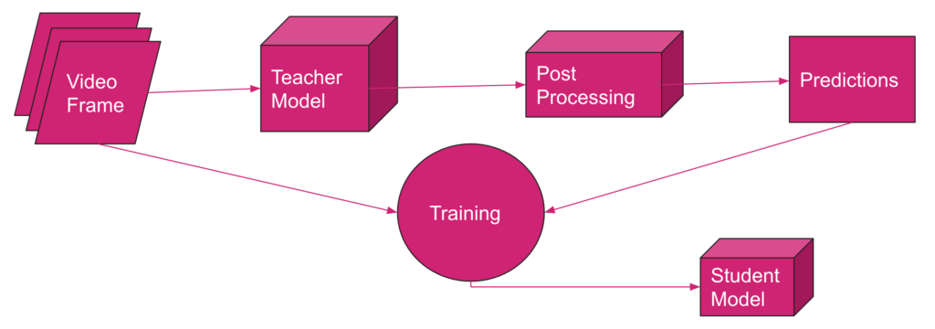
The solution consists of two phases and works as follows:
4.1. Phase One: Training
In this phase, we go through these three steps:
STEP 1: We train a heavy, complex model to do the detection task. We call this model the Teacher Model (the reason behind this naming will be clear shortly). To train the teacher model, we need to have a rich, diverse dataset and design the model complex enough to perform well on data gathered from unseen environments. This step may take some time, but it only needs to be done once. For our pedestrian detection task, we used the IterDet model pre-trained on the Crowd Human dataset. This network acts as a teacher model for new environments.
STEP 2: We feed the new environment’s data to the teacher model to get the corresponding predictions. Here, we assume that the predictions are accurate enough to be used as ground truth labels for our images. Now, we have pairs of images and labels for each frame in our input video.
STEP 3: Using the pair of images and labels from STEP 2, we train a small, lightweight model on our edge device. We refer to this model as the Student Model.
4.2. Phase Two: Inference
We can now use the student model to run the application on our edge device with high accuracy. The teacher model can now be removed from the user’s computer to free up the disk storage.
The whole adaptive learning process is illustrated in Figure 1. The training phase includes several rounds. For each round, we store a constant amount of data, say C frames, on the hard disk of the user’s computer. Then, we feed these C frames to the teacher model and obtain the corresponding labels to form C pairs of video frames and their labels. We will then use these C pairs of labeled data to train the student model. We remove these C pairs of data from the storage after they are loaded in the training pipeline and proceed to the next batch of frames, continuing from the last training checkpoint in every round.
4.3. Why Adaptive Learning?
There are several reasons why adaptive learning is a desirable solution to this problem. Here we mention some of the most important arguments:
1- Privacy: This is the first and most important reason. With adaptive learning, the teacher model runs on the user’s computer, and the student model runs on the edge device. So, everything is being processed locally, and no data needs to be stored permanently anywhere or transferred over the internet. Therefore, this approach preserves the user’s privacy and is completely safe.
2- No data annotation: By implementing this solution, you do not need to spend money and time on data annotation because the teacher model generates the labels automatically.
3- Speed: The lightweight student model is deployable on edge devices and runs in real-time, latency-free.
4- Accessibility: The most time-consuming part of adaptive learning is the training phase. However, the training phase only needs to be done once, and it takes a couple of days (at most) to finish. Afterward, we will have a lightweight model that runs on edge devices and is accessible everywhere.
To conclude, if the teacher model performs well, there is no bias in model predictions, and the student model trains well on data, adaptive learning works great.
You can find some benchmarks in Table 2 that measure mAP before and after applying adaptive learning to our pedestrian detection problem. For this example, we used the first 4500 frames of the video from the Oxford Town Centre dataset. We split these 4500 frames into training and validation sets with 3500 and 1000 frames in each set, respectively. The student model is trained on the first 3500 frames. Both baseline and adaptive learning student models are tested on the validation set with 1000 frames (from #3500 to #4500). Note that the student model is trained using the labels generated by the teacher model.
| Method | mAP | Model |
|---|---|---|
| Baseline | 25.02 | SSD-MobileNet-V2 (trained on COCO) |
| Adaptive Learning | 65.26 | Teacher: IterDet (trained on Crowd Human), Student: SSD-MobileNet-V2 |
5. Challenges
We faced several challenges when we were trying to implement adaptive learning for our application. In this section, we mention some of these challenges and share the solutions we found.
5.1. Privacy Issues Related to Storing User Data
As we mentioned earlier, for each round, we feed C images (frames) to the teacher model to get the labels for each image. Since we want to use these C pairs of images and labels in the next step to train the student model, we should temporarily store these C pairs of labeled data on the user’s computer. Choosing a large value for C results in storing a large set of user’s data on storage for each round, consuming limited resources on edge and increasing privacy risks; on the other hand, assigning a small value to C leads to catastrophic forgetting, which brings us to the next challenge.
Through trial and error, we set C to an optimal value that prevents catastrophic forgetting while keeping the number of temporarily stored images low. Note that C is the number of frames that we are storing in each round, and these frames will be deleted from the user’s computer when loaded in the training pipeline.
We also applied some tricks to the code to get the most training out of the C selected frames. For example, we only keep those frames with a number of detected objects higher than a fixed threshold to end up with a rich set of training data while avoiding storing useless data. By applying all these techniques, we could build a minimal training set that is temporarily stored on the edge device, which minimizes privacy risks and concerns.
5.2. Catastrophic Forgetting
From Wikipedia,
Catastrophic interference, also known as catastrophic forgetting, is the tendency of an artificial neural network to completely and abruptly forget previously learned information upon learning new information.
Since we are training the student model in an online and incremental manner, the network is prone to catastrophic forgetting. To put it in simple terms, we are training the model in several rounds, and in each round, the model may forget what it has learned in the earlier rounds.
In an extreme case, suppose that we are training the model on data gathered from different hours of the day, and we are feeding the data to the model in chronological order. The network may simply forget the features it has learned from images taken in daylight when it reaches the night-time images.
We should especially be aware of catastrophic forgetting when applying online learning methods to a problem. According to the last section, the value that we choose for C can give rise to or avoid catastrophic forgetting. To further mitigate this issue, we can use an adaptive learning rate and reduce the learning rate in each round as the training progresses.
5.3. Network Instabilities
The model should train even on an ordinary computer with no GPU and no big RAM as an accessible solution. Thus, we need to apply several tricks to limit the training costs. For example, we should avoid using a large batch size because larger batch sizes require more memory. However, a small batch size creates network instabilities and causes some fluctuations in the training loss and training accuracy curves.
You can reduce the learning rate to keep the batch size small while avoiding fluctuations. In our case, when we trained the network with a batch size equal to one, we got the following mAP curve:
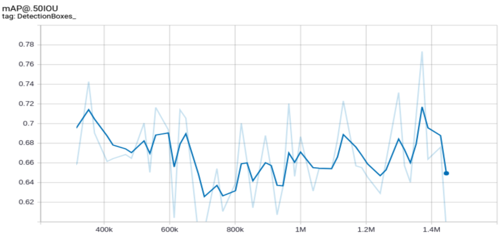
But after decreasing the learning rate, the curve was smoothed, as we see in the following figure:
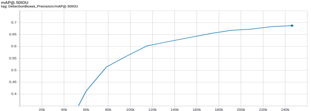
Although this approach works, it requires more time to converge. We suggest using gradient accumulation for faster convergence.
6. Improve the Accuracy Even More
So far, we have treated each frame as a separate image and processed the images independently rather than considering the temporal relation between the video frames. However, since the ultimate goal of this work is to process video feeds, taking the temporal dependencies into account during the training phase can increase accuracy.
We conducted three different experiments to enter the temporal relation between video frames into the training process by manipulating the input image’s RGB channels.
Note that there are lots of methods and model architectures in the literature that can capture temporal dependencies in video feeds in a sophisticated way. However, due to the model architecture limitations on edge (lightweight and easy to deploy on various edge devices), we could not use these methods and needed to apply other techniques to meet these limitations.
6.1. Background Subtraction:
In object detection applications where the objects of interest are moving, such as the Smart Social Distancing case, we can create a higher-level abstraction to detect the moving objects more efficiently using background subtraction. This pre-processing technique eliminates the estimated background from each frame to extract the moving objects (see Figure 4).
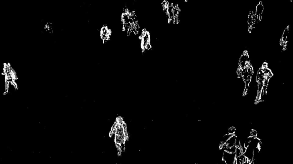
As you can see in the image above, by applying this algorithm, a mask is obtained that is active in pixels where the objects of interest (pedestrians) are present and inactive in other pixels.
To add this mask to the learning process, we replaced one of the RGB channels of the model’s input with this foreground mask.
6.2. Optical Flow
One of the most popular approaches to motion modeling in video feeds is the optical flow method.
We applied a dense optical flow algorithm to each video frame that returns the angle and magnitude of the flow vectors for each frame.
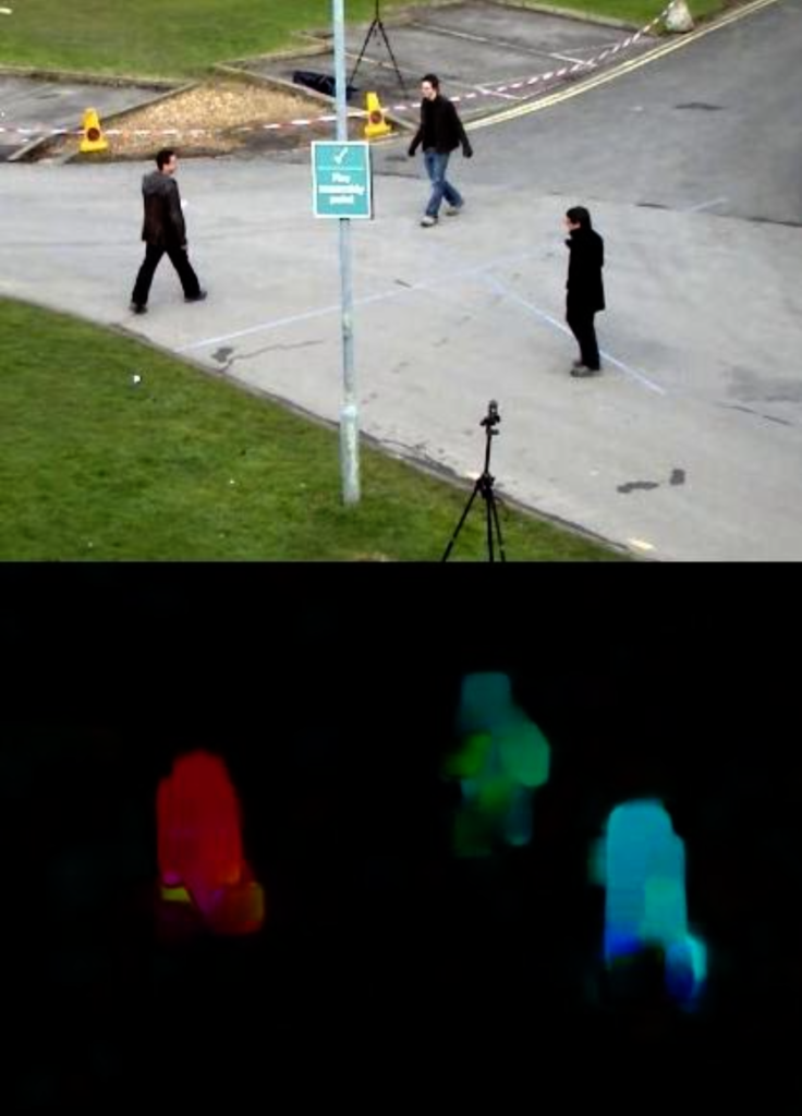
Since the angle of motion is not important in the object detection task, we discard this information and only keep the magnitude of the motion vector of each pixel in the form of a matrix. We embed the matrix of magnitudes into one of the RGB channels of the model’s input and train the student model with this supplementary information.
6.3. Combination of Background Subtraction and Optical Flow
In our last experiment, we combined the two previous techniques so that we embedded the foreground mask to one RGB channel of the model input and set the optical flow magnitude to another. For the remaining channel, we used the grayscale image of each frame to discard some color biases.
As you can see in Table 3, applying adaptive learning with background subtraction and optical flow can improve the mAP score by up to 72.2%, compared to the 25% mAP score at the baseline.
| Model | mAP Score (%) |
|---|---|
| Adaptive learning with background subtraction | 71.98 |
| Adaptive learning with optical flow | 70.56 |
| Adaptive learning with gray scale image, background subtraction, and optical flow | 72.20 |
7. Conclusion
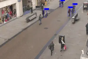
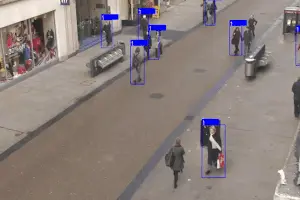
When designing the Smart Social Distancing application at Galliot, we applied Adaptive Learning to run the pedestrian detector in new environments. The results were impressive. You can compare the videos below to see the improvements (comparing the baseline on the left with adaptive learning on the right).
Suppose you need to do object detection in different environments. In that case, you can implement an adaptive learning method with a teacher-student configuration and train the student model for each environment separately. The student model will learn from the labels generated by the teacher model, so it relies on how accurately the teacher model labels the data. Aside from making sure that the teacher model labels the data with high accuracy, you need to solve several other challenges along the way, such as privacy issues related to storing user data, catastrophic forgetting, and network instabilities. Applying background subtraction and optical flow can further improve accuracy by ~7%.
You can get in touch with us for the Adaptive Learning API service and build your specialized object detection models easily. Feel free to contact us through the section provided below or via hello@galliot.us to ask for the service and further questions.
Further Readings
1- What is Gradient Accumulation in Deep Learning?
This blog post explains the backpropagation process of a neural network and the technical details of gradient accumulation, with an example provided.
2- IterDet GitHub Repository
IterDet is an iterative and self-supervised approach for improving object detection performance by leveraging unlabeled data.
3- Continual Lifelong Learning with Neural Networks: A Review
The article discusses the challenges of lifelong learning for machine learning and neural network models and compares existing approaches to alleviate catastrophic forgetting or interference. It also explores research inspired by lifelong learning factors in biological systems, such as memory replay and multisensory integration.
4- Knowledge Distillation
The blog post explains the concept of knowledge distillation, a technique that involves transferring knowledge from a larger, more complex neural network to a smaller, simpler one while maintaining its accuracy. It discusses the benefits, challenges, and applications of this technique.
5- Self-Supervised Learning and Computer Vision
Discusses the concept of self-supervised learning in machine learning and how it can be used to improve model performance. It also introduces some new techniques for self-supervised learning and provides examples of how they can be applied to real-world problems.
Also, don’t forget to check out Galliot’s GitHub repo for more information.
Quantization of TensorFlow Object Detection API Models

Image Source: https://www.deviantart.com/dnobody/art/8-Bit-Last-Supper-176002023
This tutorial explains approaches to quantization in deep neural networks and the advantages and disadvantages of using each method with a real-world example.
You can find Galliot’s Docker Containers and the required codes for this work in this GitHub Repo.
Along with optimization methods, high-quality datasets can make a huge difference in your deep learning model’s performance. Read more about Data Labeling Methods, Challenges, and Tools to create better datasets.
Check out Galliot’s other Services and Solutions.
In this tutorial, we will examine various TensorFlow tools for quantizing object detection models. We start off by giving a brief overview of quantization in deep neural networks, followed by explaining different approaches to quantization and discussing the advantages and disadvantages of using each approach. We will then introduce TensorFlow tools to train a custom object detection model and convert it into a lightweight, quantized model with TFLiteConverter and TOCOConverter. Finally, as a use case example, we will examine the performance of different quantization approaches on the Coral Edge TPU.
Quantization in Neural Networks: the Concept
Quantization, in general, refers to the process of reducing the number of bits that represent a number. Deep neural networks usually have tens or hundreds of millions of weights, represented by high-precision numerical values. Working with these numbers requires significant computational power, bandwidth, and memory. However, model quantization optimizes deep learning models by representing model parameters with low-precision data types, such as int8 and float16, without incurring a significant accuracy loss. Storing model parameters with low-precision data types not only saves bandwidth and storage but also results in faster calculations.
Quantization brings efficiency to neural networks
Quantization improves overall efficiency in several ways. It saves the maximum possible memory space by converting parameters to 8-bit or 16-bit instead of the standard 32-bit representation format. For instance, quantizing the Alexnet model shrinks the model size by 75%, from 200MB to only 50MB.
Quantized neural networks consume less memory bandwidth. Fetching numbers in the 8-bit format from RAM requires only 25% of the bandwidth of the standard 32-bit format. Moreover, quantizing neural networks results in 2x to 4x speedup during inference.
Faster arithmetics could be another benefit of quantizing neural networks in some cases, depending on different factors, such as the hardware architecture. As an example, 8-bit addition is almost 2x faster than 64-bit addition on an Intel Core i7 4770 processor.
These benefits make quantization valuable, especially for edge devices that have modest computing and memory but are required to perform AI tasks in real-time.
Quantizing neural networks is a win-win
By reducing the number of bits that represent a parameter, some information is lost. However, this loss of information incurs little to no degradation in the accuracy of neural networks for two main reasons:
1- This reduction in the number of bits acts like adding some noise to the network. Since a well-trained neural network is noise-robust, i.e., it can make valid predictions in the presence of unwanted noises, the added noise will not degrade the model accuracy significantly.
2- There are millions of weight and activation parameters in a neural network that are distributed in a relatively small range of values. Since these numbers are densely spread, quantizing them does not result in losing too much precision.
To give you a better understanding of quantization, we next provide a brief explanation of how numbers are represented in a computer.
Computer representation of numbers
Computers have limited memory to store numbers. There are only discrete possibilities to represent the continuous spectrum of real numbers in the representation system of a computer. The limited memory only allows a fixed amount of values to be stored and represented in a computer, which can be determined based on the number of bits and bytes the computer representation system works with. Therefore, representing real numbers in a computer involves an approximation and a potential loss of significant digits.
There are two main approaches to storing and representing real numbers in modern computers:
1. Floating-point representation: The floating-point representation of numbers consists of a mantissa and an exponent. In this system, a number is represented in the form of mantissa * base exponent, where the base is a fixed number. In this representation system, the position of the decimal point is specified by the exponent value. Thus, this system can represent both very small values and very large numbers.
2. Fixed-point representation: In this representation format, the position of the decimal point is fixed. The numbers share the exponent, and they vary in the mantissa portion only.
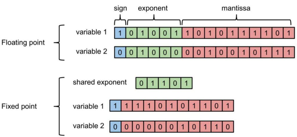
Figure 1. Floating-point and fixed-point representation of numbers (image source).
The amount of memory required for the fixed-point format is much less than the floating-point format since the exponent is shared between different numbers in the former. However, the floating-point representation system can represent a wider range of numbers compared to the fixed-point format.
The precision of computer numbers
The precision of a representation system depends on the number of values it can represent precisely, which is 2b, where b is the number of bits. For example, an 8-bit binary system can represent 28 = 256 numbers precisely. In this system, only 256 values are represented precisely. The rest of the numbers are rounded to the nearest number of these 256 values. Thus, the more bits we can use, the more precise our numbers will be.
It is worth mentioning that the 8-bit representation system in the previous example is not limited to representing integer values from 1 to 256. This system can represent 256 pieces of information in any arbitrary range of numbers.
How to quantize numbers in a representation system
When quantizing numbers in a representation system, some numbers are represented precisely, and some are approximated by the closest quantized value. To determine the representable numbers in a representation system with brr2b to find uk * uk = 0, 1, ..., 255rk -> k * uk * u(k + 1) * u
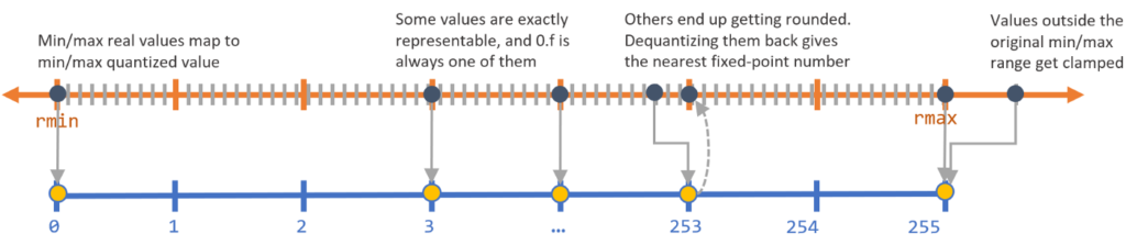
Figure 2. Quantizing numbers in a representation system (image source).
In the next section, we will explain how we can calculate the range of parameters in a neural network in order to quantize them.
How to quantize neural networks
Quantization is to change the current representation format of numbers to another lower precision format by reducing the amount of the representing bits. In machine learning, we use the floating-point format to represent numbers. By applying quantization, we can change the representation to the fixed-point format and down-sample these values. In most cases, we convert the 32-bit floating-point to the 8-bit fixed-point format, which gives almost 4x reduction in memory utilization.
There are at least two sets of numerical parameters in each neural network; the set of weights, which are constant numbers (in inference) learned by the network during the training phase, and the set of activations, which are the output values of activation functions in each layer. By quantizing neural networks, we mean quantizing these two sets of parameters.
As we saw in the previous section, to quantize each set of parameters, we need to know the range of values each set holds and then quantize each number within that range to a representable value in our representation system. While finding the range of weights is straightforward, calculating the range of activations can be challenging. As we will see in the following sections, each quantization approach deals with this challenge in its own way.
Most of the quantization techniques are applied to inference but not training. The reason is that in each backpropagation step of the training phase, parameters are updated with changes that are too small to be tracked by a low-precision data-type. Therefore, we train a neural network with high-precision numbers and then quantize the weight values.
Types of Neural Network Quantization
There are two common approaches to neural network quantization: 1) post-training quantization and 2) quantization-aware training. We will next explain each method in more detail and discuss the advantages and disadvantages of each technique.
Post-training quantization
The post-training quantization approach is the most commonly used form of quantization. In this approach, quantization takes place only after the model has finished training.
To perform post-training quantization, we first need to know the range of each parameter, i.e., the range of weights and activations. Finding the range of weights is straightforward since weights remain constant after training has been finished. However, the range of activations is challenging to determine because activation values vary based on the input tensor. Thus, we need to estimate the range of activations. To do so, we provide a dataset that represents the inference data to the quantization engine (the module that performs quantization). The quantization engine calculates all the activations for each data point in the representative dataset and estimates the range of activations. After calculating the range of both parameters, the quantization engine converts all the values within those ranges to lower bit numbers.
The main advantage of using this technique is that it does not require any model training or fine-tuning. You can apply 8-bit quantization on any existing pre-trained floating-point model without using many resources. However, this approach comes at the cost of losing some accuracy because the pre-trained network was trained regardless of the fact that the parameters will be quantized to 8-bit values after training has been finished, and quantization adds some noise to the input of the model at inference time.
Quantization-aware training
As we explained in the previous section, in the post-processing quantization approach, training was in floating-point precision regardless of the fact that the parameters would be quantized to lower bit values. This difference of precision that originates from quantizing weights and activations enters some error to the network that propagates through the network by multiplications and additions.
In quantization-aware training, however, we attempt to artificially enter this quantization error into the model during training to make the model robust to this error. Note that similar to post-training quantization, in quantization-aware training, backpropagation is still performed on floating-point weights to capture the small changes.
In this method, extra nodes that are responsible for simulating the quantization effect will be added. These nodes quantize the weights to lower precision and convert them back to the floating-point in each forward pass and are deactivated during backpropagation. This approach will add quantization noise to the model during training while performing backpropagation in floating-point format. Since these nodes quantize weights and activations during training, calculating the ranges of weights and activations is automatic during training. Therefore, there is no need to provide a representative dataset to estimate the range of parameters.
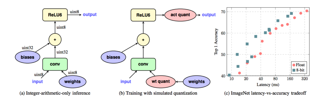
Figure 3. Quantization-aware training method (image source).
Quantization-aware training gives less accuracy drop compared to post-training quantization and allows us to recover most of the accuracy loss introduced by quantization. Moreover, it does not require a representative dataset to estimate the range of activations. The main disadvantage of quantization-aware training is that it requires retraining the model.
Here you can see benchmarks of various models with and without quantization.
Model Quantization with TensorFlow
So far, we have described the purpose behind quantization and reviewed different quantization approaches. In this section, we will dive deep into the TensorFlow Object Detection API and explain how to perform post-training quantization and quantization-aware training.
TensorFlow object detection API
The TensorFlow Object Detection API is a framework for training object detection models that offers a lot of flexibility. You can quickly train an object detector in three steps:
STEP 1: Change the format of your training dataset to tfrecord
STEP 2: Download a pre-trained model from the TensorFlow model zoo.
STEP 3: Customize a config file according to your model architecture.
You can learn more about each step in the TensorFlow Object Detection API GitHub repo.
Figure 4. TensorFlow Object Detection API (image source).
This tool provides developers with a large number of pre-trained models that are trained on different datasets, such as COCO. Therefore, you do not need to start from scratch to train a new model; you can simply retrain the pre-trained models for your specific needs.
Object Detection API offers various object detection model architectures, such as SSD and Faster-RCNN. We trained an SSD Lite MobileNet V2 model using the TensorFlow Object Detection API on the Oxford Town Centre dataset to build a pedestrian detection model for the Smart Social Distancing application. We picked the SSD architecture to be able to run this application in real-time on different edge devices such as NVIDIA Jetson Nano and Coral Edge TPU. We used ssdlite_mobilenet_v2_coco.config
Note that TensorFlow 1.12 or higher is required for this API, and this API does not support TensorFlow 2.
Installing TensorFlow object detection API with Docker
Installing Object Detection API can be time-consuming. Instead, you can use Galliot’s Docker container to get TensorFlow Object Detection API installed with minimal effort.
This Docker container will install the TensorFlow Object Detection API and its dependencies in the /models/research/object_detection
1- Run with CPU support:
- Build the container from the source:
# 1- Clone the repository
git clone https://github.com/neuralet/neuralet
cd training/tf_object_detection_api

# 2- Build the container
docker build -f tools-tf-object-detection-api-training.Dockerfile -t "neuralet/tools-tf-object-detection-api-training" .

# 3- Run the container
docker run -it -v [PATH TO EXPERIMENT DIRECTORY]:/work neuralet/tools-tf-object-detection-api-training
- Pull the container from Docker Hub:
docker run -it -v [PATH TO EXPERIMENT DIRECTORY]:/work neuralet/tools-tf-object-detection-api-training
2- Run with GPU support:
You should have the Nvidia Docker Toolkit installed to be able to run the docker container with GPU support.
- Build the container from the source:
# 1- Clone the repository
git clone https://github.com/neuralet/neuralet cd training/tf_object_detection_api

# 2- Build the container
docker build -f tools-tf-object-detection-api-training.Dockerfile -t "neuralet/tools-tf-object-detection-api-training" .

# 3- Run the container
docker run -it --gpus all -v [PATH TO EXPERIMENT DIRECTORY]:/work neuralet/tools-tf-object-detection-api-training
- Pull the container from Docker Hub:
docker run -it --gpus all -v [PATH TO EXPERIMENT DIRECTORY]:/work neuralet/tools-tf-object-detection-api-training
Exporting the model to a frozen graph
After training the model, you can find the trained checkpoints, i.e., .ckptprotobuf file by freezing its computational graph. In general, you can use the export_inference_graph.pytfliteexport_tflite_ssd_graph.py
python3 object_detection/export_tflite_ssd_graph.py \
 --pipeline_config_path=$CONFIG_FILE \
 --trained_checkpoint_prefix=$CHECKPOINT_PATH \
 --output_directory=$OUTPUT_DIR \
 --add_postprocessing_op=true
Running this script will create a .pb$OUTPUT_DIR
Post-training quantization with TFlite Converter
As described earlier, post-training quantization allows you to convert a model trained with floating-point numbers to a quantized model. You can apply post-training quantization using TFlite Converter to convert a TensorFlow model into a TensorFlow Lite model that is suitable for on-device inference.
This API provides three options to quantize a floating-point 32-bit model to lower precisions:
1. quantize only weights to 8-bit precision
2. quantize both weights and activations to 8-bit precision
3. quantize only weights to floating-point 16-bit precision
We will investigate the first two approaches in this tutorial. Quantizing to floating-point 16-bit precision is beyond the scope of this article. Read this guide for more detail.
Weight quantization of a retrained SSD MobileNet V2
After exporting the model to a frozen graph, you can quantize the model weights by running the following Python script:
[1] import tensorflow as tf
[2] frozen_graph_file = # path to frozen graph (.pb file)
[3] input_arrays = ["normalized_input_image_tensor"]
[4] output_arrays = ['TFLite_Detection_PostProcess',
[5]           'TFLite_Detection_PostProcess:1',
[6]           'TFLite_Detection_PostProcess:2',
[7]           'TFLite_Detection_PostProcess:3']
[8] input_shapes = {"normalized_input_image_tensor" : [1, 300, 300, 3]}
[9]
[10] converter = tf.lite.TFLiteConverter.from_frozen_graph(frozen_graph_file,
[11]                                                  input_arrays=input_arrays,
[12]                                                  output_arrays=output_arrays,
[13]                                                  input_shapes=input_shapes)
[14] converter.allow_custom_ops = True
[15] converter.optimizations = [tf.lite.Optimize.DEFAULT]
[16] tflite_quant_model = converter.convert()
[17] with open(tflite_model_quant_file, "wb") as tflite_file:
[18]     tflite_file.write(tflite_model_quant)
You only need to set the path to the frozen graph file and change the input shape. You can leave the rest of the code as it is.
In line 2.pb
In lines 3-8
In lines 10-13
Line 14allow_custom_ops14, you tell the TFLite Converter to find and quantize those registered custom operations. This line will raise an error in case of failure. Read more on custom operations and how to register them here.
In line 15
Finally, in lines 16-18.tflite
Note that in this method, TensorFlow Lite quantizes some of the activations dynamically in inference time in addition to weight quantization to improve model latency.
Full Integer Quantization of a Retrained SSD MobileNet V2
We now explain how to quantize the full network, including weights, activations, inputs, and outputs to 8-bit numbers.
Run the following script to perform full 8-bit quantization:
[1] import tensorflow as tf
[2] frozen_graph_file = # path to frozen graph
[3] input_arrays = ["normalized_input_image_tensor"]
[4] output_arrays = ['TFLite_Detection_PostProcess',
[5]     'TFLite_Detection_PostProcess:1',
[6]     'TFLite_Detection_PostProcess:2',
[7]     'TFLite_Detection_PostProcess:3']
[8] input_shapes = {"normalized_input_image_tensor" : [1, 300, 300, 3]}
[9] converter = tf.lite.TFLiteConverter.from_frozen_graph(saved_model_dir,input_arrays,
[10]     output_arrays, input_shapes)
[11] converter.allow_custom_ops = True
[12] converter.optimizations = [tf.lite.Optimize.OPTIMIZE_FOR_SIZE]
[13] converter.representative_dataset = _representative_dataset_gen
[14] tflite_model_quant = converter.convert()
[15] with open(tflite_model_quant_file, "wb") as tflite_file:
[16]     tflite_file.write(tflite_model_quant)
This script is similar to the last one, except that a representative_dataset
[1] import cv2
[2] import numpy as np
[3] from imutils import paths
[4] def _representative_dataset_gen():
[5]     images_path = # path to represantative dataset
[6]     if images_path is None:
[7]         raise Exception(
[8]             "Image directory is None, full integer quantization requires images directory!"
[9]         )
[10]     imagePaths = list(paths.list_images(images_path))
[11]     for p in imagePaths:
[12]         image = cv2.imread(p)
[13]         image = cv2.cvtColor(image, cv2.COLOR_BGR2RGB)
[14]         image = cv2.resize(image, (300, 300))
[15]         image = image.astype("float")
[16]         image = np.expand_dims(image, axis=1)
[17]         image = image.reshape(1, 300, 300, 3)
[18]         yield [image.astype("float32")]
As you can see in this example, you should specify the path to sample images that represent the input data used in inference time. Based on our experience, a dataset of ~100 images would be enough for the TFLite Converter to reach an accurate estimate of the range of the activations.
Important Notes:
1. Those operations that are not supported by the TFLite Converter remain in floating-point after post-training quantization. If you want the converter to throw an error if an operation does not quantize, you should add the following line of code to your script: converter.target_spec.supported_ops = [tf.lite.OpsSet.TFLITE_BUILTINS_INT8]
2. If you want the converter to quantize the inputs and outputs of the model, add the following lines to the code:converter.inference_input_type = tf.uint8 & converter.inference_output_type = tf.uint8
Note that if you are quantizing your object detection model using the current version of the TensorFlow Lite Converter, adding these two lines of code will fail the quantization due to some compatibility issues.
Quantization-aware training with TensorFlow object detection API
You can use the TensorFlow Model Optimization Tool to perform quantization-aware training for Keras-based models. You can use this tool in either of two ways: 1- specify some layers to be quantized-aware, or 2- set the whole model to be quantized-aware. You can install this tool by following the installation guide here.
However, if you are using the TensorFlow Object Detection API to train your model, you cannot use TensorFlow Model Optimization Tool for quantization-aware training. This is because the current version of the object detection API requires TensorFlow 1.x, which is not compatible with the model optimization tool. To apply quantization-aware training for object detection models that are trained using the object detection API, you need to make some config changes.
If you take a look at the sample config files of the object detection API, you will notice some files that contain the quantized keyword in their name, such as the ssd_mobilenet_v2_quantized_300x300_coco.configgraph_rewriter
graph_rewriter {
  quantization {
  delay: 48000
  weight_bits: 8
  activation_bits: 8
  }
}
By adding these lines to your config file, you tell TensorFlow that you want to perform quantization-aware training. The delay
The other two parameters specify the number of bits that weights and activations will be quantized to. Only 8-bit quantization is supported by TensorFlow at this time.
You can start quantization-aware training from a quantized or non-quantized pre-trained model checkpoint. See the object detection model zoo to explore object detection models and their checkpoints. For the pedestrian detection task, we used the ssd_mobilenet_v2_quantized_300x300_coco.configssd_mobilenet_v2_coco
After training has been finished, we can freeze the model and export the frozen graph by running the export_tflite_ssd_graph.py
TOCO
So far, we have trained a floating-point model by simulating the quantization effect in the training process, but we have not quantized the model yet. TensorFlow offers another tool that quantizes a model and exports it to a tflite
Based on TensorFlow documentation, to quantize your object detection model with TOCO, you need to build TensorFlow from the source. This can be a daunting procedure since it is time-consuming and may lead to environment inconsistencies that fail the build after a long process. To overcome this issue, we created an easy-to-use docker container. This container takes in the frozen graph file path and some other specifications as parameters and generates the tflite
Model quantization using the TOCO Docker container
To quantize your model using Galliot’s TOCO Docker container, you can either build the container from the source or pull the container from Docker Hub.
- Build the container from the source:
# 1- Clone the repository
git clone https://github.com/neuralet/neuralet cd training/tf_object_detection_api

# 2- Build the container
docker build -f tools-toco.Dockerfile -t "neuralet/tools-toco" .

# 3- Run the container
docker run -v [PATH_TO_FROZEN_GRAPH_DIRECTORY]:/model_dir neuralet/tools-toco --graph_def_file=[frozen graph file]
- Pull the container from Docker Hub:
docker run -v [PATH_TO_FROZEN_GRAPH_DIRECTORY]:/model_dir neuralet/tools-toco --graph_def_file=[frozen graph file]
After running the container, you can find the quantized object detection model named detect.tflite in FROZEN_GRAPH_DIRECTORY
You can also customize other parameters when running the docker container. For example, you can override the default input shape and inference type by giving --input_shapes=[DEFAULT:1,300,300,3]--inference_type=[DEFAULT:QUANTIZED_UINT8]
Quantization Example: Coral Edge TPU
In this section, we deploy an object detection model on a Coral Edge TPU device to illustrate one of the applications of model quantization.
Edge TPU only supports 8-bit weights and activations; thus, we first need to quantize our model to 8-bit precision to be able to work with the device. We have described three strategies for quantizing an SSDlite MobileNet V2 model:
1. post-training quantization of weights
2. post-training quantization of weights and activations
3. quantization-aware training and quantization of weights and activations
Since Edge TPU requires 8-bit quantized parameters, the first strategy does not apply to these devices because activations remain in floating-point following this approach. We will now explain model quantization using the next two methods on an Edge TPU device.
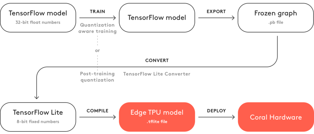
Figure 5. Steps required to deploy a TensorFlow model on edge TPU (image source).
To deploy a model on an Edge TPU device, you need to compile the quantized tflite
Operator                       Count      Status

CUSTOM                         1          Operation is working on an unsupported data type
ADD                            10         Mapped to Edge TPU
CONCATENATION                  2          Mapped to Edge TPU
QUANTIZE                       11         Mapped to Edge TPU
CONV_2D                        55         Mapped to Edge TPU
DEPTHWISE_CONV_2D              33         Mapped to Edge TPU
DEQUANTIZE                     2          Operation is working on an unsupported data type
RESHAPE                        13         Mapped to Edge TPU
LOGISTIC                       1          Mapped to Edge TPU
For each operator, this log displays the operator name, the number of operators in the model, and the operator status, which indicates whether that operator is mapped to edge TPU or it will run on the CPU.
The log file for quantization-aware training is as follows:
Operator                       Count      Status

CUSTOM                         1          Operation is working on an unsupported data type
ADD                            10         Mapped to Edge TPU
CONCATENATION                  2          Mapped to Edge TPU
CONV_2D                        55         Mapped to Edge TPU
DEPTHWISE_CONV_2D              33         Mapped to Edge TPU
RESHAPE                        13         Mapped to Edge TPU
LOGISTIC                       1          Mapped to Edge TPU
As you can see, the two DEQUANTIZE
Now we feed the Oxford Town Centre dataset to the compiled models and compute the latency and frame rate on the Coral Dev Board. The results are as follows:
| Quantization Approach | Inference Time [ms] | Frame Rate [FPS] |
|---|---|---|
| post-training quantization | 6.6 | 152 |
| quantization-aware training | 6.1 | 164 |
Visit Galliot’s GitHub repository for more examples of Edge TPU inferencing.
Conclusion
Quantization allows us to convert object detection models trained in floating-point numbers to lightweight models with lower-bit precisions. Quantized models accelerate calculations and consume less memory; therefore, they are ideal for edge computing applications.
In the Smart Social Distancing application, we have applied quantization to our pedestrian detection model to increase the speed of model inference and be able to run our application on different edge devices in real-time.
Visit Galliot’s GitHub repository for more projects. You can also reach us by email at hello@galliot.com.
A quick review of what we have explained in this article:
1- What is the Low-Bit Quantization of Neural Networks?
The process of reducing the bits that represent a number is called Quantization in general. When it comes to Deep Neural Networks (DNNs), we are talking about millions of high-precision numerical values (bits) as model weights. To process these gigantic amounts of numbers, we require significant computational power, processors, memory, and bandwidth. While quantizing our DNNs, we are actually optimizing our Deep Learning models by representing their parameters with low-precision data types such as int8 or float16 without causing significant accuracy loss. This optimization saves much bandwidth and storage and brings about faster calculations.
2- What are the upsides and drawbacks of Quantization in Neural Networks?
Upsides: It Saves Memory, Requires less Memory and Bandwidth, and yields Faster Arithmetic.
Downsides: Quantization lets a Noise enter the Neural Network that might affect and degrade the model’s accuracy. The noise is an error produced by low-precision arithmetic and approximations.
3- What are the differences between post-training quantization and quantization-aware training”?
Post-Training Quantization happens right after finishing the model’s training. Most significantly, it requires no model training or fine-tuning. Plus, you won’t need many resources to apply 8-bit quantization on an existing pre-trained floating-point model. However, due to adding some noise into the network, this approach costs you to lose some accuracy.
In Quantization-Aware Training, we anticipate and consider the error quantizing the weights may add to the network. Then, we try to artificially enter this error into the model during the training and make the model robust to this quantization error.
4- How to use TensorFlow tools to Train and Quantize an Object Detection model?
TensorFlow Object Detection API offers a lot of flexibility for training object detection models. This framework presents lots of pre-trained models trained on various datasets like COCO. So, instead of starting from scratch, you will be able to use its available models and retrain them based on your particular use case.
Since TFLite models are more appropriate for on-device inference, the TFLite Converter will allow you to apply post-training quantization and transform a TensorFlow model into a TFLite version.
To conduct Quantization-Aware training for Keras-based models, the TensorFlow Model Optimization is a practical tool for you.
TensorFlow offers another tool that quantizes a model and exports it to a tflite
5- How to convert an Object Detection model for Coral Edge TPU:
First, you should create a quantized TFLite version of the model. Note that since the Edge TPU only supports 8-bit integer arithmetic, full integer quantization should be performed on the model. Then you can compile this TFLite model for Edge TPU by Edge TPU Compiler (edgetpu_compiler
Further Readings
1- 8-Bit Quantization and TensorFlow Lite
This blog post explores the concept of 8-bit quantization and how it can be used with TensorFlow Lite to speed up mobile inference with low precision.
2- TensorFlow Object Detection API
This is the readme file of the TensorFlow Object Detection API repository on GitHub. The file contains information on how to use the API for training, evaluation, and deployment of object detection models.
3- Quantization Aware Training with TensorFlow Model Optimization Toolkit
The blog post explains how to use the TensorFlow Model Optimization Toolkit for Quantization Aware Training, which allows for training models with reduced precision to improve speed and decrease memory usage without losing accuracy.
4- TensorFlow Post-Training Integer Quantization
The post introduces the addition of post-training integer quantization to the Model Optimization Toolkit, a suite of techniques used to optimize machine learning models for deployment and execution. Integer quantization reduces the numerical precision of the weights and activations of models, improving memory and latency.
5- Quantization and Training of NNs for Efficient Integer-Arithmetic-Only Inference
The article proposes an on-device inference scheme that uses integer-only arithmetic to improve efficiency and reduce computational costs. The improvements were tested on MobileNets and demonstrated in ImageNet classification and COCO detection on popular CPUs.